Indiana's Housing Market in 2014:

Indiana Association of REALTORS

Indiana’s Housing Market in 2014:

December

2014

Moving toward Stability

Prepared for

Indiana’s Housing

Market in 2014:

Moving toward Stability

December 2014

Prepared for

Indiana Association of REALTORS

Matt Kinghorn, Economic Analyst

Indiana Business Research Center,

Kelley School of Business, Indiana University

Table of Contents

EXECUTIVE SUMMARY .................................................................................................... 1

Key Findings .............................................................................................................................................. 2

MARKET CONDITIONS .................................................................................................... 3

Pace of Home Sales Cools in 2014 .......................................................................................................... 3

Indiana’s Median Sales Price Makes a Large Leap in 2013 ......................................................................................................... 5

Indiana House Prices in Perspective ........................................................................................................ 7

Foreclosure Wave Begins to Recede...................................................................................................... 10

Implications of High Foreclosure Rates ...................................................................................................................................... 12

Looking Ahead ........................................................................................................................................ 14

DEMOGRAPHIC FUNDAMENTALS .................................................................................... 18

Population Growth and Household Formation on the Upswing .............................................................. 18

Indiana’s Homeownership Rate Continues to Slide ................................................................................ 21

Looking Ahead ........................................................................................................................................ 22

HOUSING AND THE ECONOMY ........................................................................................ 25

Residential Construction Improving, but Still Weak ................................................................................ 25

Housing’s Impact on Employment ........................................................................................................... 26

Looking Ahead ........................................................................................................................................ 27

CONCLUSION .............................................................................................................. 30

APPENDIX ................................................................................................................... 31

Home Sales and Median Sales Price by County, Year-over-Year Change, July 2013 to June 2014 ......................................... 31

Number of Units and Value of Residential Building Permits by County, 2012 to 2013 ............................................................... 33

Housing Affordability Index Methodology .................................................................................................................................... 35

iii

Index of Figures

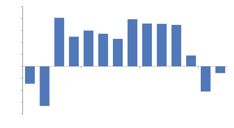
Figure 1: Indiana Home Sales, Year-over-Year Change, 2011:1 to 2014:2 ........................................................................................... 4

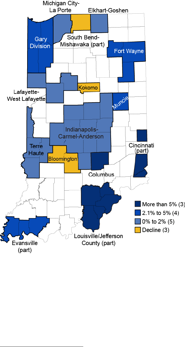
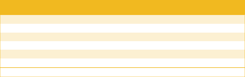
Figure 2: Total Home Sales by Metro Area, Year-over-Year Change, July 2013 to June 2014 ............................................................. 5

Figure 3: Indiana Median Sales Price, 2005 to 2013 .............................................................................................................................. 6

Figure 4: Median Sales Price and Months' Supply, 12-Month Moving Average, January 2007 to June 2014 ....................................... 7

Figure 5: Change in House Price Index by State, 2013:2 to 2014:2 ....................................................................................................... 8

Figure 6: House Price Index, 1991:1 to 2014:2 ...................................................................................................................................... 8

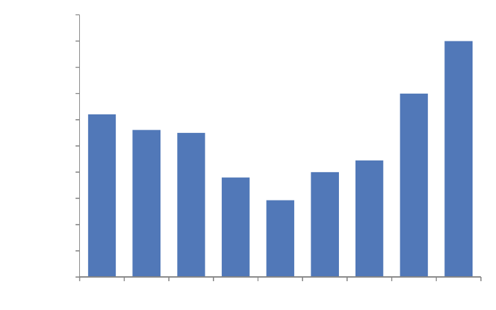
Figure 7: Average Annualized Growth in HPI over Select Periods, 1991:1 to 2014:2 ............................................................................ 9

Figure 8: Ratio of Median Sales Price to Median Household Income, 1991 to 2013............................................................................ 10

Figure 9: Share of Mortgages in Foreclosure, 1979:1 to 2014:2 .......................................................................................................... 11

Figure 10: FHA and Subprime Loans as a Share of All Mortgages and Foreclosure Inventory, 2014:2 ............................................. 12

Figure 11: Indiana Foreclosure Rate and Year-over-Year Change in House Price Index, 1992:1 to 2014:2 ....................................... 13

Figure 12: Indiana Existing Home Sales and Single-Family Housing Permits, 1988 to 2013 .............................................................. 14

Figure 13: Indiana Employment and Unemployment Rate Forecast, 2013:1 to 2017:4 ....................................................................... 15

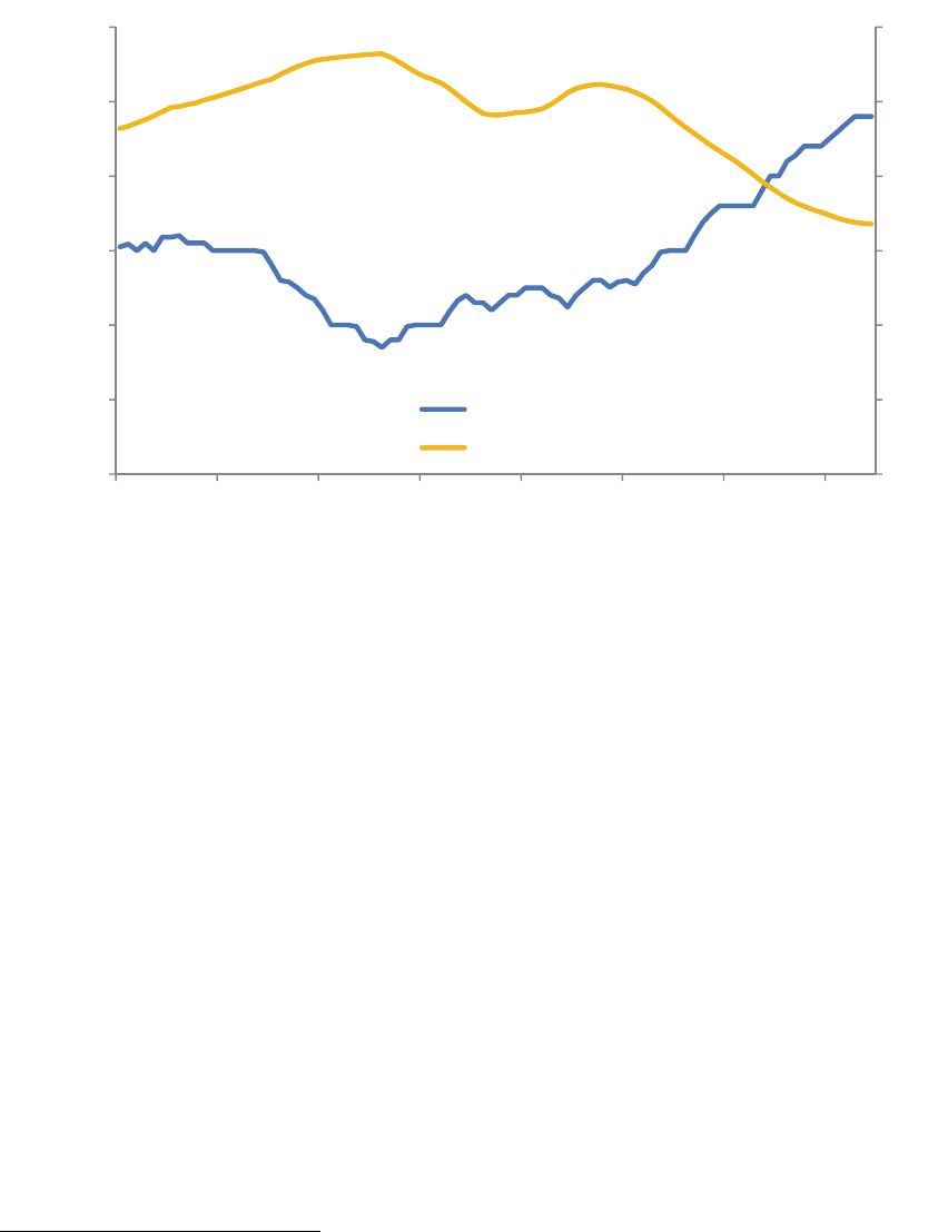
Figure 14: Mortgage Interest Rates and Indiana Housing Affordability Index, January 1979 to June 2014 ........................................ 16

Figure 15: Indiana Annual Population Change, 1983 to 2013 .............................................................................................................. 18

Figure 16: Comparison of Net Migration Estimates for Suburban Counties of Select Metro Areas ..................................................... 19

Figure 17: Average Annual Household Formation Rates, 1990 to 2013 .............................................................................................. 20

Figure 18: Indiana Homeownership Rates by Age, 2000 to 2013 ........................................................................................................ 22

Figure 19: Indiana Population Projections by Age, 2010 to 2020 ......................................................................................................... 23

Figure 20: U.S. Residential Fixed Investment and Indiana Value of Building Permits, 1991 to 2013 ................................................. 26

Figure 21: Indiana Homeowner and Rental Vacancy Rates, 2006 to 2013 .......................................................................................... 27

Figure 22: U.S. Total Home Equity Cashed Out and Personal Savings Rate, 1993:1 to 2014:2 ........................................................ 28

Index of Tables

Table 1: Indiana Housing Market by the Numbers .................................................................................................................................. 1

Table 2: Indiana Existing Home Sales, 2006 to 2013 ............................................................................................................................. 3

Table 3: Estimated Shortfall in Number of Indiana Households in 2013............................................................................................... 21

Contact Information

For more information about this report, contact the Indiana Business Research Center at

(812) 855-5507 or email [email protected].

Executive Summary

Indiana has seen dramatic improvement in many key housing market indicators over the last couple of

years. Existing home sales improved by 31 percent between 2011 and 2013 and the state’s foreclosure

rate has dropped to its lowest level since early 2001. Indiana house prices have regained nearly all the

ground lost during the slump, and even residential construction—although still well below historic norms—

has shown signs of life.

So far in 2014, however, price gains and construction activity have moderated some, and existing home

sales have taken a step back. Odd as it may sound though, these developments could also be seen as

positive signs since they likely signal a move toward normalcy in housing. That is, for at least a decade,

Indiana’s housing markets have been overly influenced by a series of national-level forces. Factors like

easy lending practices, the Great Recession, federal homebuyer tax credits, historically low mortgage

rates and bulk home purchases by investors have fueled booms and busts in local markets.

In 2014, these influences are either long gone or at least fading, which has helped to dampen some

housing-related activity lately. Moving forward, the ups and downs in housing indicators are likely to be

less dramatic as local markets increasingly sink or swim on the strength of their own economic and

demographic fundamentals.

Table 1: Indiana Housing Market by the Numbers

U.S. Indiana

Existing Home Sales, July 2013 to June 2014, Year-over-Year Change 1.4% 2.0%

House Price Appreciation, 2013:2 to 2014:2 6.2% 3.7%

Residential Building Permits, July 2013 to June 2014, Year-over-Year Change 8.1% 16.6%

Share of Mortgages That Are Seriously Delinquent, 2014:2 4.8% 5.2%

Share of Mortgages with Negative Equity, 2014:2 10.7% 5.1%

Household Formation Rate, 2013 0.3% 0.7%

Sources: Indiana Association of Realtors, National Association of Realtors, Federal Housing Finance Agency, U.S. Census Bureau,

Mortgage Bankers Association and CoreLogic

Fortunately, Indiana’s fundamentals appear to be improving. As of August 2014, the state has added

more than 58,000 jobs in the last year, and its unemployment rate has dropped 1.7 percentage points.

Indiana had the nation’s sixth-best improvement in median household income in 2013 according to the

Current Population Survey, and its per capita income growth has outpaced the U.S. average over the last

few years. After an extended period of sluggish population growth, the state had a relatively strong net in-

migration of residents in 2013, and its household formation rate last year was on par with pre-recession

levels. Finally, mortgage rates did spike in 2013 but they remain very low, and research by the Federal

Reserve indicates that lending standards for prime loans may be loosening a bit.

The Indiana housing market has made great strides in recent years, but these gains were more about

playing catch-up and were often ahead of market fundamentals. Now that the drivers of housing demand

are improving, the state may be poised for a period of steady but sustainable housing market growth.

This report examines some of the latest data in order to gauge the state of Indiana’s housing market. The

first section presents a detailed overview of market conditions with a focus on home sales and prices,

mortgage delinquency and foreclosure, and affordability. The next section examines the demographic

drivers of the housing market, including household formation rates, migration and the aging population.

Finally, we consider the role of housing in Indiana’s economy with a look at construction activity and

mortgage refinancing trends.

Key Findings

 Existing home sales in Indiana increased by 14 percent in 2013, the state’s second consecutive year

of double-digit increases. The number of sales declined so far this year, however. Through the first

half of 2014, existing home sales are down 6 percent compared to the same period a year ago.

 Indiana’s median price for existing home sales rose to $122,000 in 2013—a 3 percent increase over

the previous year and 11 percent above 2009. The Federal Housing Finance Agency’s House Price

Index shows that Indiana had the 29

-fastest rate of price appreciation among states in the last year.

 Indiana’s foreclosure rate has declined dramatically of late, dropping to its lowest level in 13 years.

The state’s foreclosure rate has dropped by nearly 2.4 percentage points between the end of 2011

and mid-2014 to 2.5 percent. Over this period, Indiana has gone from the nation’s ninth-highest

foreclosure rate to 18

-highest.

 According to the most recent census data, Indiana’s homeownership rate declined from 71.4 percent

in 2000 to 68.5 percent in 2013. Despite this drop, Indiana had the 13

-highest homeownership rate

in the country and was well above the U.S. mark of 63.5 percent.

 The aging of the baby boomers into the prime age group for homeownership helps to mask what is an

even more dramatic drop in homeownership. In 2013, the homeownership rates for each 10-year age

group between the ages of 25 and 64 were down by between 5 and 8 percentage points compared to

Census 2000. Under normal conditions, Indiana’s homeownership rate would have risen over this

period simply because the state is growing older and homeownership increases with age.

 Housing affordability conditions have declined some as house prices and mortgage rates climb, but

housing in Indiana remains very affordable by any objective standard. According to Moody’s

Economy.com, Indiana enjoyed the nation’s third-best housing affordability conditions in 2013.

 After five years of very sluggish growth between 2006 and 2011, Indiana’s household formation rate

has been rising the last two years. The state’s formation rate hit 0.7 percent in 2013, which was more

than two-times greater than the U.S. mark—and equal to Indiana’s average annual rate prior to the

housing slump. A relatively strong net in-migration of residents to the state in 2013 helped to boost

household formation last year.

 For the fourth consecutive year, the value of Indiana’s building permits increased in 2013. This is

good news, yet construction has fallen to such an extent that the value of permits in 2013—even

when measured in nominal terms (i.e., not adjusted for inflation)—was a shade below the level seen

in 1994.

 The number of new housing units permitted for construction in 2013 climbed 30 percent over the

previous year. Apartment developments accounted for roughly 30 percent of these new units—the

highest multi-family share since 1986. Despite this strong increase, 2013 marks Indiana’s 11th-lowest

annual number of permitted units since 1960. Growth in permits has slowed to 6 percent year-over-

year through July 2014.

Market Conditions

Pace of Home Sales Cools in 2014

Indiana had its second consecutive year of strong gains in existing home sales home in 2013. The state’s

sales tally last year was up 14 percent over the 2012 mark and was its strongest annual figure since 2007

(see Table 2). Furthermore, Indiana had roughly 18,000 more existing home sales in 2013 than it did

during its post-recession low in 2010.

Table 2: Indiana Existing Home Sales, 2006 to 2013

2006 2007

2008

2009

2010

2011 2012

2013

Existing Home Sales 86,142 79,545 66,505 61,826 57,765 57,985 66,516 75,849

Annual Percent Change n/a -7.7% -16.4% -7.0% -6.6% 0.4% 14.7% 14.0%

Source: Indiana Association of Realtors

As Figure 1 shows, however, the rebound in existing home sales slowed significantly in late 2013 and

has reversed some during the first half of this year. Existing home sales in Indiana during the first quarter

of 2014 were nearly 11 percent lower than during the same period a year ago. Meanwhile, sales in the

second quarter were down three percent year-over-year.

There are several factors that contribute to this recent decline in home sales. The two largest are likely a

rise in mortgage interest rates and a decline in home purchases by investor groups.

The 30-year

conventional mortgage rate jumped a full percentage point between May and December of last year and,

while it has declined some this year, it remains quite a bit higher than it was in 2012 and the first half of

2013. As for investors, several media reports in 2013 showed that they played a role in the home sales

rebound in some Indiana markets by buying a large number of single family homes and converting them

into rental properties.

But as prices climb and the stock of foreclosed homes declines rapidly, investor

purchases have likely been on the wane in Indiana this year, as they have been around the country.

John Krainer, “The Slowdown in Existing Home Sales,” Federal Reserve Bank of San Francisco, May 2014,

http://www.frbsf.org/economic-research/publications/economic-letter/2014/may/existing-home-sales-slowdown/

Jeff Swiatek, “Indianapolis Official Wary of Investor Groups Snapping Up Homes,” Indystar.com, September 4, 2013.

“Q2 2014 U.S. Institutional Investor and Cash Sales Report,” RealtyTrac, August 2014, www.realtytrac.com/content/foreclosure-

market-report/q2-2014-us-institutional-investor-and-cash-sales-report-8126

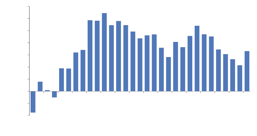
Figure 1: Indiana Home Sales, Year-over-Year Change, 2011:1 to 2014:2

Source: Indiana Association of Realtors

Considering these factors then, the recent dip in home sales is not necessarily a sign of a weakening

market, but more likely signals a stabilizing one. The nearly 34,700 home sales through the first half of

2014 are still the state’s second-highest total for this period since 2007. The number of sales remains well

below levels seen last decade before the crash but, of course, that was a period of easy financing and an

abnormally high homeownership rate in Indiana (along with a comparatively high foreclosure rate). It

doesn’t seem likely—or even desirable—that Indiana will see sales totals that high anytime soon. Instead,

the state’s sales totals will be more closely tied to economic and demographic fundamentals as the

influence of factors like low interest rates and investor buying diminishes.

Looking at local markets for a 12-month period ending in June 2014, the Indiana portions of the Louisville

and Cincinnati metro areas had the state’s greatest increases in existing home sales with gains of 10

percent and 9 percent, respectively (see Figure 2). The Columbus area also posted a strong jump in

sales with a 7 percent improvement year-over-year. The 11-county Indianapolis-Carmel-Anderson metro,

which accounts for 30 percent of the state’s total population, claimed 38 percent of Indiana’s home sales

over this period.

-20%

-15%

-10%

-5%

10%

15%

20%

25%

2011 2012 2013 2014

Figure 2: Total Home Sales by Metro Area, Year-over-Year Change, July 2013 to June 2014

Source: Indiana Association of Realtors

The 48 counties that are outside of metro areas combined to post a 1 percent increase in sales. Among

counties with at least 100 sales, Jay County had the largest increase at 40 percent followed by Perry (26

percent), Jennings (23 percent) and Wabash (21 percent) counties.

Statewide, sales are up roughly 2

percent over this period.

Indiana’s Median Sales Price Makes a Large Leap in 2013

As the market for existing homes in Indiana stabilizes, house prices are on the climb. At $122,000 last

year, the state’s median sales price for existing homes increased by more than 3 percent over the 2012

See the appendix for home sales and median sales price data for all Indiana counties.

mark and was 11 percent above the low point in 2009 (see Figure 3). Furthermore, according to data

from the Indiana Association of Realtors that dates to 2004, the median sales price in 2013 is the state’s

highest annual mark on record.

Figure 3: Indiana Median Sales Price, 2005 to 2013

Source: Indiana Association of Realtors

The sharp increase in prices over the last two years has been driven in large part by a shrinking inventory

of homes for sale. As of June 2014, the inventory of homes for sale in Indiana was slightly greater than

44,100. This is 16 percent lower than for the same month in 2012 and 42 percent lower than the inventory

in June 2007.

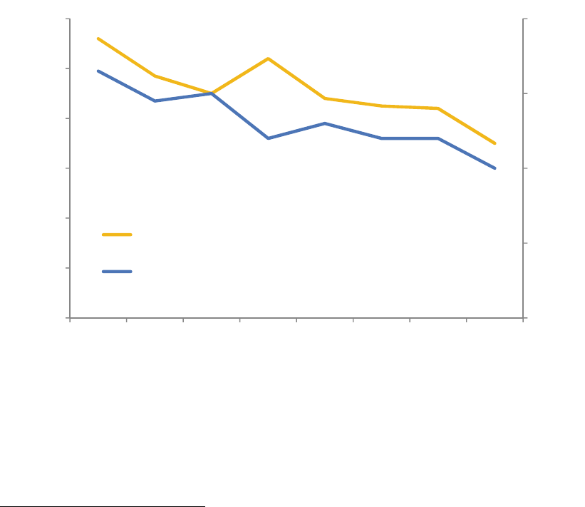
The decline in inventory coupled with an uptick in demand has led to a seven-year low in the estimated

months’ supply of existing homes for sale in Indiana. The months’ supply measure is an estimate of how

long it would take to work through the inventory of homes for sale in a given month at the average

monthly sales rate over the previous year. As one would expect, there is a strong negative relationship

between months’ supply and prices (correlation = -0.93), with prices increasing as supply began to drop

steadily in 2011 (see Figure 4).

$104

$106

$108

$110

$112

$114

$116

$118

$120

$122

$124

2005 2006 2007 2008 2009 2010 2011 2012 2013

Median Sales Price (thousands)

Figure 4: Median Sales Price and Months' Supply, 12-Month Moving Average, January 2007

to June 2014

Source: Indiana Association of Realtors

Indiana’s median sales price has climbed to $124,000 over the 12-month period ending in June 2014—a

3.3 percent increase year-over-year. Looking around the state over the same period, the median sales

price held steady or increased in 63 of Indiana’s 92 counties. Among the state’s larger markets, Hamilton

(8 percent increase), Hendricks (7.8 percent), Grant (7.7 percent), St. Joseph (7.3 percent) and

Bartholomew (7 percent) counties posted the largest increases over this 12-month period. Madison (-5.3

percent), Floyd (-4.1 percent), and Vigo (-3.9 percent) counties had the largest price declines among

communities with at least 500 existing home sales.

Indiana House Prices in Perspective

Other measures show that Indiana’s house prices are improving as well. According to the Federal

Housing Finance Agency’s House Price Index (HPI), Indiana has seen price appreciation for ten

consecutive quarters dating back to early 2012 and the state’s home prices in the second quarter of 2014

are up 3.7 percent year-over-year.

This rate of appreciation ranked 29

-fastest among states but was

outpaced by neighboring Michigan (10.3 percent), Ohio (7.8 percent) and Illinois (4.2 percent). Indiana did

edge out Kentucky, which had an HPI increase of 3.6 percent over this period. As Figure 5 illustrates,

several of the hardest-hit states during the crash posted the greatest gains led by Nevada (15.8 percent)

and California (15.3 percent).

An HPI like this one from FHFA is conceptually different from the median sales price indicator discussed earlier. Comparing the

median sales price from one period to another can be misleading since the median price is influenced by the mix of homes sold in

each period. The HPI is a repeat-sales index, meaning that it measures the changes in sales price when a given property is sold

multiple times. This approach removes a good deal of the comparability problems inherent in the median sales price.

$100

$105

$110

$115

$120

$125

$130

2007 2008 2009 2010 2011 2012 2013 2014

Months

In Thousands

Median Price (left axis)

Months' Supply of Inventory (right axis)

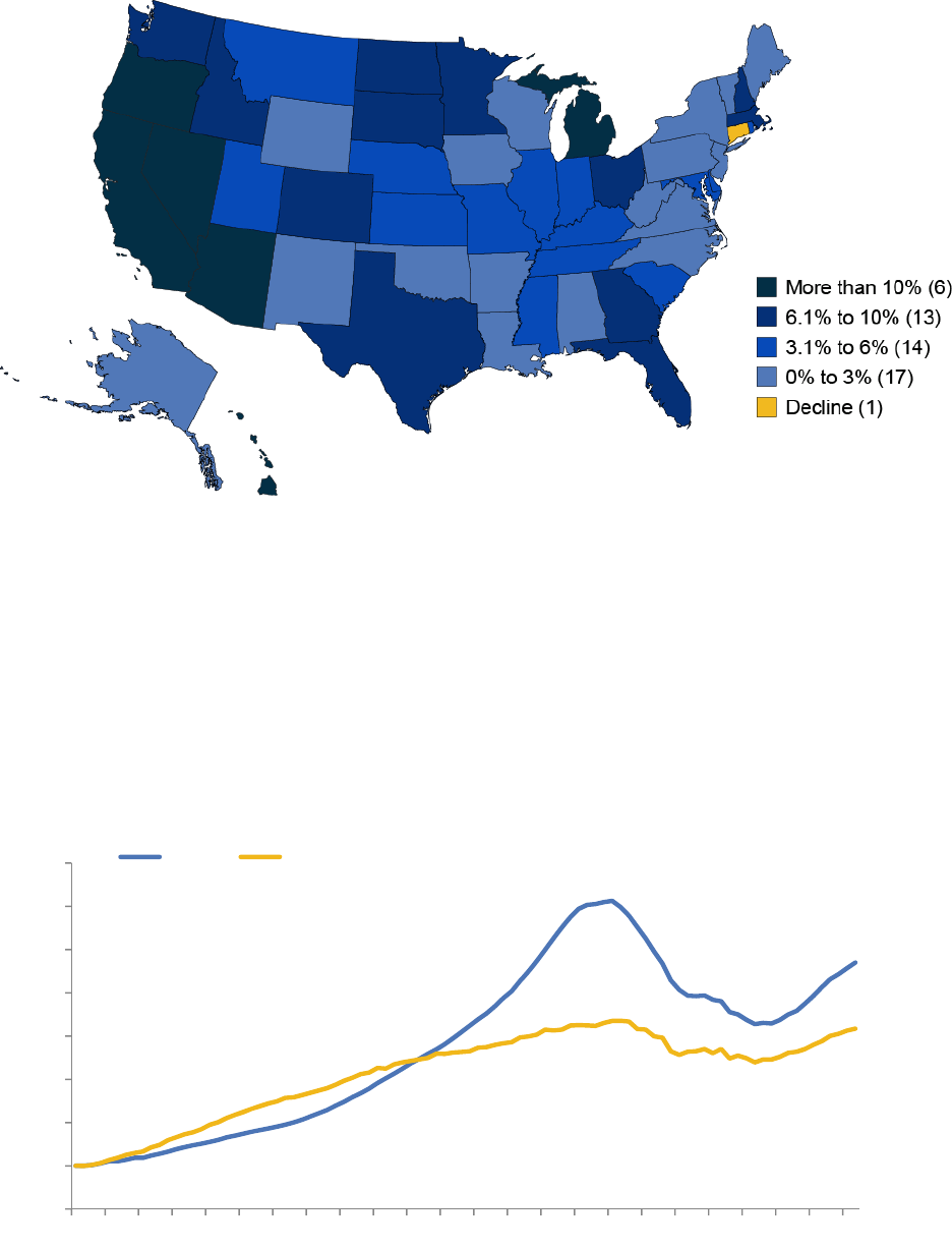
Figure 5: Change in House Price Index by State, 2013:2 to 2014:2

Source: Federal Housing Finance Agency, House Price Index (expanded data series, seasonally adjusted)

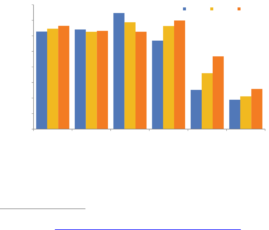
It is important to note that comparing states based on one-year growth rates can be a little misleading.

States like Michigan, Ohio and Illinois are outpacing Indiana now because they are rebounding from far

more severe price declines through the housing bust. House prices in Michigan declined by 45 percent

after the crash. Ohio and Illinois saw drops of 25 percent and 32 percent, respectively. Indiana had a

comparatively mild 12 percent slide in prices between 2007 and 2011. Since that time, the state has

recovered nearly all the ground it lost (see Figure 6). As of mid-2014, the HPI for Indiana was only 2

percent lower than its pre-recession peak. House prices in Michigan and Illinois, by contrast, are both still

more than 25 percent below their respective peaks, and Ohio is 14 percent off its previous high.

Figure 6: House Price Index, 1991:1 to 2014:2

Source: Federal Housing Finance Agency, House Price Index (expanded data series, seasonally adjusted)

100

120

140

160

180

200

220

240

1991 1993 1995 1997 1999 2001 2003 2005 2007 2009 2011 2013

U.S. Indiana

Looking at the previous graphic, it’s easy to see that both Indiana and the U.S. have undergone four

distinct periods of house price appreciation trends over the past 25 years. The Hoosier state saw

comparatively strong gains during much of the 1990s, but its pace of growth began to slow just as the

price bubble era started to emerge elsewhere. Prices began to decline in Indiana and the U.S. in 2007,

but both have had a sustained rebound in effect since early 2012.

During this rebound period, prices in Indiana have been growing at an average annualized rate of 3.4

percent—which is much stronger than the pace the state set between 2000 and 2007 and not far off the

trend of the 1990s (see Figure 7). Nationally, the HPI growth rate during the recent rebound is near the

unsustainable pace set before the crash—which has raised some concerns that the U.S. could be headed

for another bubble. This concern appears overblown, however—at least for the time being. A recent

analysis by the real estate website Trulia estimates that prices in the U.S. on average are still slightly

undervalued.

Furthermore, the pace of HPI growth has been slower so far in 2014 than it was the year

before, and it should continue to moderate as inventory expands.

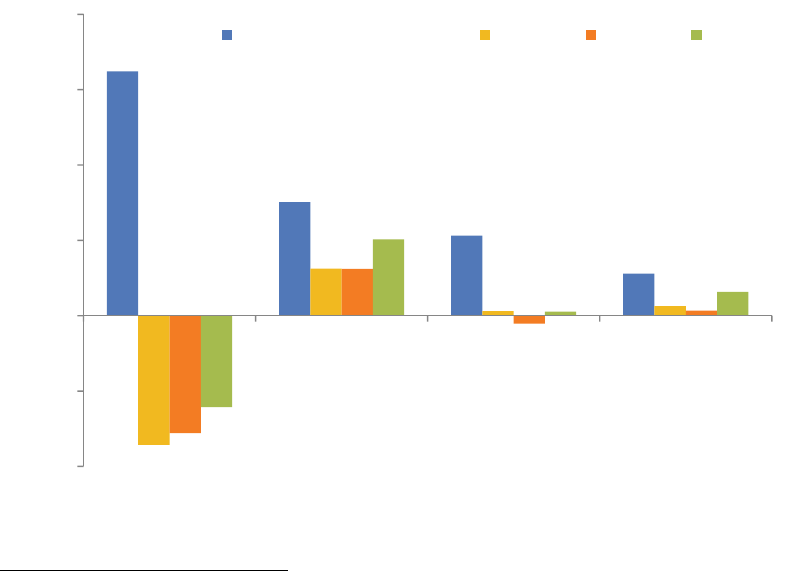
Figure 7: Average Annualized Growth in HPI over Select Periods, 1991:1 to 2014:2

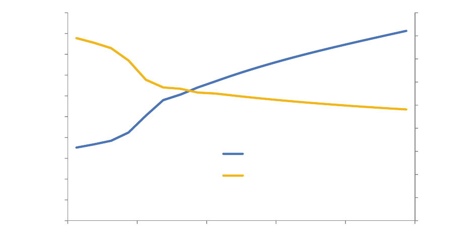
Here in Indiana, there is no concern over a price bubble. One enduring characteristic of Indiana housing

is that the movement of most key market indicators are closely tied to the state’s economic performance.

The ratio of the state’s median sales price to median household income may be the best illustration of this

point. The U.S. had a consistent ratio of house prices to income through the 1990s, but this measure

increased sharply between 2000 and 2005 (see Figure 8). Since the onset of the housing slump,

however, the U.S. price-to-income ratio tumbled back to the more sustainable level seen during the

1990s—although, as discussed earlier, the spike in 2013 does merit some concern.

Jed Kolko, “Bubble Watch: Home Prices Still Undervalued, But Not For Much Longer,” Trulia Trends, June 24, 2014,

www.trulia.com/trends/2014/06/bubble-watch-q2-2014/.

3.4%

6.4%

-5.8%

5.9%

4.1%

2.0%

-2.4%

3.4%

-8%

-6%

-4%

-2%

U.S. Indiana

2000:1 to 2007:21991:1 to 1999:4

2007:3 to 2011:4

2012:1 to 2014:2

All the while, through a relative boom period in the 1990s and two recessions during the 2000s, Indiana’s

ratio has held remarkably steady over the last two decades. Even with the strong jump in the state’s

median sales price in 2013, Indiana had an increase in median household income to match. According to

the U.S. Census Bureau, Indiana’s median income improved by nearly 10 percent in 2013 to $50,550—

the sixth-best increase among states last year.

Figure 8: Ratio of Median Sales Price to Median Household Income, 1991 to 2013

Source: U.S. Census Bureau and Moody’s Economy.com

Foreclosure Wave Begins to Recede

One of the primary ways that economic conditions have influenced home prices in recent years was

through the dramatic rise in foreclosures. For instance, the mortgage technology firm FNC Inc. reports

that, at the depth of the crisis in early 2009, roughly 37 percent of all U.S. home sales were foreclosed

properties. At the same time, these foreclosures were selling at 25 percent below market value.

As the foreclosure situation improved, its effect on prices has diminished. At the national level,

foreclosures as a share of sales had been cut by nearly three-quarters to 10.5 percent by July 2014.

Furthermore, FNC indicates that the foreclosure discount has fallen to 8 percent during the second

quarter of 2013, which is a ten-year low in this measure.

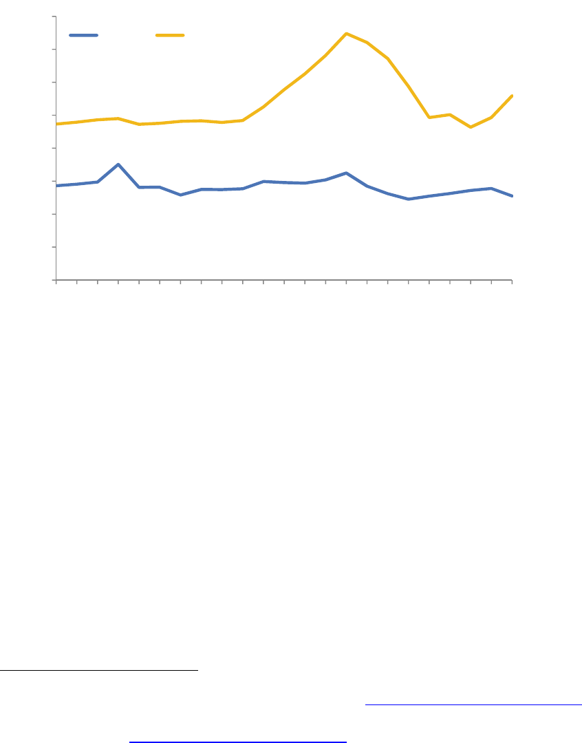
This situation should continue to improve as the volume of lender-owned properties decline in Indiana

and around the country. Figure 9 shows that the state has seen a sharp drop in its foreclosure rate since

the end of 2011. According to the Mortgage Bankers Association, the state’s foreclosure rate has

declined nearly two-and-a-half percentage points from 4.96 in the fourth quarter of 2011 to 2.54 in mid-

“FNC Index: July Home Prices Up 0.6%,” FNC Inc., September 16, 2014, http://fncrpi.com/press_releases.aspx?pr=84.

“Amid Rapid Declines of Foreclosure Rates and Rising Prices, Prospective Trade-Up Buyers Are Returning to the Market,” FNC

Inc., September 12, 2013, http://fncrpi.com/press_releases.aspx?pr=69.

1.0

1.5

2.0

2.5

3.0

3.5

4.0

4.5

5.0

1991 1993 1995 1997 1999 2001 2003 2005 2007 2009 2011 2013

Ratio

Indiana U.S.

2014. This is Indiana’s lowest quarterly foreclosure rate since early 2001. Even with this dramatic decline,

Indiana’s foreclosure rate remains slightly above the U.S. average and ranks 18

-highest among states.

Figure 9: Share of Mortgages in Foreclosure, 1979:1 to 2014:2

Source: National Delinquency Survey, Mortgage Bankers Association

One reason that Indiana has struggled with a high foreclosure rate for the last 13 years is that Hoosiers

are more reliant on high-risk mortgages. In the second quarter of 2014, 27 percent of Indiana’s

outstanding mortgages were so-called FHA loans.

An additional 9 percent of the state’s mortgages were

subprime. When combined together, Indiana had the nation’s second-largest share (behind Oklahoma) of

these types of loans at 36 percent of all mortgages. By contrast, FHA loans (17 percent) and subprime

loans (9 percent) combine to account for 26 percent of all U.S. mortgages, according to the Mortgage

Bankers Association.

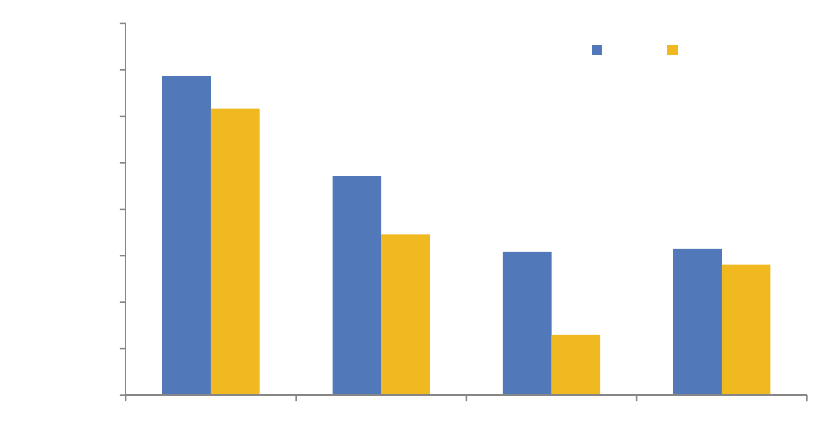
In Indiana, 3.2 percent of FHA loans were in foreclosure in mid-2014 compared to 1.5 percent of the

state’s prime mortgages. The state’s foreclosure rate for subprime loans stands at 7.7 percent, which is

lower than the U.S. mark of 9.7 percent. So while these types of loans account for a little more than one-

third of Indiana’s home loans, they represent 61 percent of Indiana’s foreclosure inventory due to their

comparatively high default rates (see Figure 10). These higher-risk loans account for 53 percent of the

foreclosure inventory nationwide.

FHA loans are loans from private lenders that are insured by the Federal Housing Administration. These loans typically feature low

down-payment requirements and are intended for borrowers who would likely not qualify for a mortgage without the insurance.

1979

1981

1983

1985

1987

1989

1991

1993

1995

1997

1999

2001

2003

2005

2007

2009

2011

2013

U.S.

Indiana

Figure 10: FHA and Subprime Loans as a Share of All Mortgages and Foreclosure

Inventory, 2014:2

Source: National Delinquency Survey, Mortgage Bankers Association

Implications of High Foreclosure Rates

Indiana’s improving foreclosure rate will have several positive effects on the state’s housing market. First,

house prices will continue to receive a boost from a shrinking foreclosure inventory. Not only do the

foreclosed properties add to the total pool of homes for sale, but they also tend to sell at a discount and

depress home values in their surrounding neighborhood.

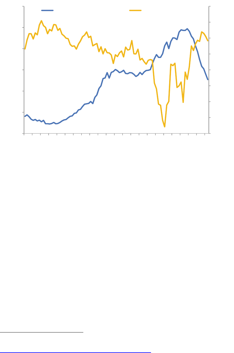
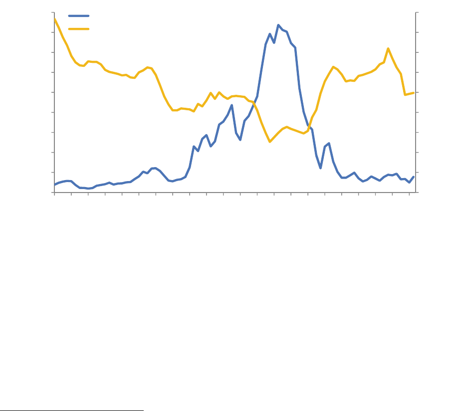
Figure 11 highlights this relationship between foreclosure and house price changes. These two measures

have a strong negative correlation (-0.73), suggesting that changes in one will influence the other—

although the causal relationship is not a one-way street.

Foreclosures affect prices for the reasons listed

above, but rising prices can also reduce the pool of homeowners at risk of foreclosure by allowing

homeowners to build equity more quickly.

Stephan Whitaker, “Foreclosure-Related Vacancy Rates,” Federal Reserve Bank of Cleveland, July 26, 2011,

www.clevelandfed.org/research/commentary/2011/2011-12.cfm.

The one time that the relationship between foreclosures and price changes did not hold was in late 2009 and early 2010 when the

federal government’s homebuyer tax credit programs temporarily boosted house prices.

10%

20%

30%

40%

50%

60%

70%

Share of All Mortgages Share of Foreclosure Inventory

U.S. Indiana

Figure 11: Indiana Foreclosure Rate and Year-over-Year Change in House Price Index,

1992:1 to 2014:2

Source: Mortgage Bankers Association, Federal Housing Finance Agency

Fewer foreclosures and rising house prices should also help spur demand for new home construction.

Before the housing crash, there was a consistent ratio of five to six existing home sales for each new

home sold at the national level. Since the beginning of 2007, however, housing demand has tilted even

more heavily toward increasingly affordable existing homes. As a result, the ratio of existing home sales

to new homes climbed to roughly 13-to-1 by mid-2014. The price discount on existing homes brought on

by foreclosures and other distressed properties at least partially explains this widening gap.

This is a

trend that the economics blog Calculated Risk has termed the “distressing gap,” referring to the large

number of distressed home sales since the start of the housing bust.

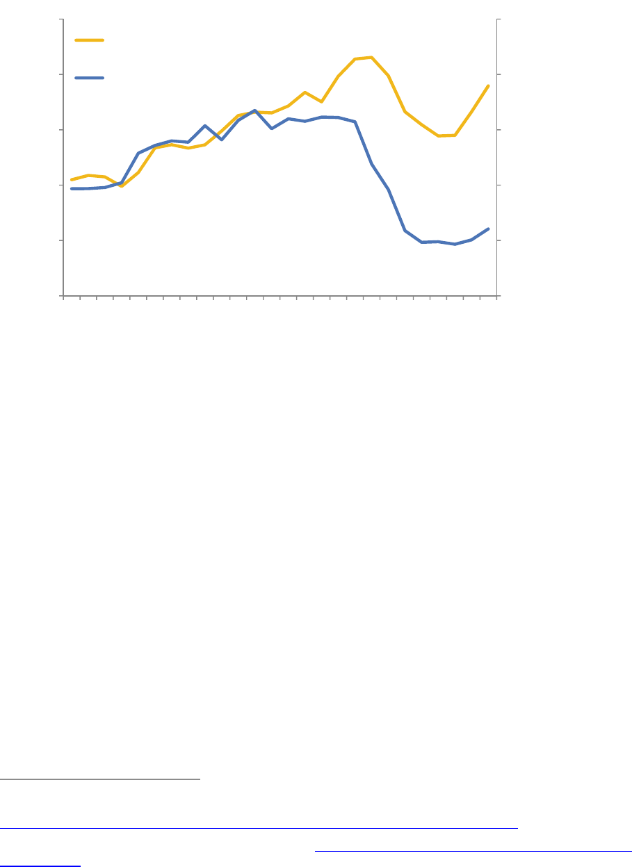
New home sales data are not available for states, so we are unable to confirm if this relationship holds in

Indiana. However, a comparison of existing home sales and annual housing construction permits

suggests that the same dynamics are at play (see Figure 12). From 1988 to 2005, there were

approximately two existing home sales for each single-family housing permit in Indiana, but in 2013 the

ratio was roughly six-to-one. As the market continues to stabilize, this gap will have to begin closing over

the next few years.

Bill McBride, “Comments on New Home Sales,” Calculated Risk (blog), August 25, 2014,

www.calculatedriskblog.com/2014/08/comments-on-new-home-sales.html.

-8%

-6%

-4%

-2%

1992 1994 1996 1998 2000 2002 2004 2006 2008 2010 2012 2014

Change in HPI

Foreclosure Rate

Foreclosure Rate (left axis) HPI Change (right axis)

Figure 12: Indiana Existing Home Sales and Single-Family Housing Permits, 1988 to 2013

Source: U.S. Census Bureau, Moody’s Economy.com

Looking Ahead

The Indiana housing market has made great strides in the last two-and-a-half years, and it should

continue to improve through 2015. Among the bright spots is the decline in Indiana’s foreclosure rate to

its lowest level since early 2001. Over the next year or two, look for the state’s foreclosure rate to

continue dropping before settling at a level well below that seen between 2002 and 2006—a period

before the Great Recession when Indiana had one of the highest foreclosure rates in the nation.

The primary reason for optimism is simply the length of time elapsed between now and the days of easy

lending. That is, with respect to the risky mortgages issued before the crash, many of those that were

destined to default have likely done so by now. Meanwhile, at the national level at least, mortgages

originated after 2008 have proven far less likely to slip into delinquency.

Thanks to stricter lending

standards, the flow of mortgages into foreclosure in Indiana has been declining since 2010, and should

continue to fall.

The state’s rising house prices will also continue to help solve the foreclosure problem. According to

CoreLogic, roughly 5 percent of Indiana homeowners with a mortgage had negative equity as of the

second quarter of 2014.

This mark is down sharply from nearly 12 percent of Hoosier homeowners with

negative equity at the beginning of 2013. Even more encouraging, one-quarter of these homeowners with

negative equity were close to getting back into an equity position (i.e., within 5 percent of home value). So

as prices rise, more and more of these (currently) underwater homeowners will be in a better position to

“Black Knight Mortgage Monitor,” Black Knight Financial Services, July 2014,

www.bkfs.com/CorporateInformation/NewsRoom/MortgageMonitor/201407/MortgageMonitorJuly2014.pdf.

“CoreLogic Equity Report,” CoreLogic, Second Quarter 2014, www.corelogic.com/research/negative-equity/corelogic-q2-2014-

equity-report.pdf .

100

1988

1990

1992

1994

1996

1998

2000

2002

2004

2006

2008

2010

2012

Housing Permits (thousands)

Existing Home Sales (thousands)

Home Sales (left axis)

Housing Permits (right axis)

avoid foreclosure in the event that they fall behind on their payments. As a point of comparison, 12.7

percent of all U.S. mortgages have negative equity.

One of the major question marks facing the market looking into 2015 revolves around the direction of

existing home sales. As discussed earlier, a combination of factors that include higher mortgage rates, a

decline in investor purchases and a harsh winter have led to year-over-year declines in existing home

sales so far this year. Although the severity of these declines has diminished in the summer months to the

point where the combined closed sales in June and July of this year are down just 0.2 percent compared

to the same months in 2012. Looking at the same periods, pending existing home sales are up 5.5

percent, however, which suggests that Indiana will see a return to year-over-year sales gains this fall.

Of course, the future path of home sales will depend on the strength of the economy and housing

affordability. The prospects for Indiana’s economy look solid. As of August 2014, Indiana has added more

than 58,000 jobs over the past 12 months. According to the latest forecast from the IBRC and the Center

for Econometric Model Research (CEMR) at Indiana University, employment growth should continue at a

pace of roughly 45,000 new jobs per year between 2015 and 2017 (see Figure 13). The state’s

unemployment rate is expected to dip below 5 percent by the end of that period, as well.

Perhaps the best economic news for Indiana is that the state is seeing relatively strong personal income

growth. The state’s per capita personal income had been losing ground to the U.S. mark in a big way

between the mid-1990s and the late 2000s, but Indiana has started to chip away at that gap over the last

six years. The latest CEMR forecast indicates that Indiana incomes will continue to gain ground on the

nation over the next three years as well.

Figure 13: Indiana Employment and Unemployment Rate Forecast, 2013:1 to 2017:4

Source: Center for Economic Model Research and Indiana Business Research Center, Indiana University (released in August 2014)

As for affordability, Indiana remains one of the most buyer-friendly markets in the country. According to

Moody’s Economy.com, Indiana enjoyed the third-best housing affordability conditions among states in

2013, ranking behind only Michigan and Ohio. As the housing market stabilizes, however, affordability is

2,750

2,800

2,850

2,900

2,950

3,000

3,050

3,100

3,150

3,200

3,250

2013 2014 2015 2016 2017

Unemployment Rate

Employment (thousands)

Employment (left axis)

Unemployment Rate (right axis)

bound to come back to earth a bit. Not only are house prices on the rise, but mortgage rates are up too

(see Figure 14). After peaking at 4.5 percent in December 2013, rates have declined slightly so far this

year, but many market-watchers expect them to start climbing again soon. In their September forecasts,

both the Mortgage Bankers Association and Freddie Mac predict the rate will hit at least the 5 percent

mark in 2015.

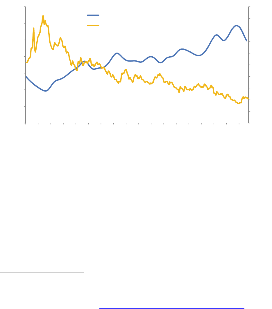
Figure 14: Mortgage Interest Rates and Indiana Housing Affordability Index,

January 1979 to June 2014

Note: An index value of 100 means that a state’s median household income is exactly enough to qualify for a mortgage on a

median-priced home. Values above 100 indicate that the median income is more than enough to qualify. Indiana’s index value was

248 in June 2014, meaning that the state’s median household income was 248 percent of the income needed for a mortgage on the

median-priced house. See the appendix for the index methodology. Monthly affordability values are interpolated from annual data.

The 2014 index values are a forecast.

Source: Freddie Mac and Moody’s Economy.com

Rising rates will certainly have a negative impact on some potential buyers, but housing in Indiana will

remain affordable by any objective standard for some time. An analysis last year by Freddie Mac

indicates that housing would remain affordable in metro areas throughout the Midwest with mortgage

rates as high as 8 percent, and they could probably go even higher before housing is considered

unaffordable (8 percent is the highest level in their analysis).

Another positive sign for home sales is that there are finally indications that mortgage lending standards

may start to loosen a bit. While it was certainly appropriate that lenders tightened standards after the

housing bust, there have been concerns that standards are too conservative and an impediment to a full

economic recovery.

According to the Federal Reserve’s latest quarterly survey of senior loan officers,

however, roughly one-quarter of respondents stated that their institutions had eased standards for prime

“What Happens When Interest Rates Rise?,” U.S. Economic & Housing Market Outlook, Freddie Mac, June 2013,

http://www.freddiemac.com/finance/pdf/Jun_2013_public_outlook.pdf .

Ben S. Bernanke, “Challenges in Housing and Mortgage Markets” (speech given at the Operation HOPE Global Financial Dignity

Summit, Atlanta, Georgia, November 15, 2012), www.federalreserve.gov/newsevents/speech/bernanke20121115a.htm.

100

150

200

250

300

350

1979 1981 1983 1985 1987 1989 1991 1993 1995 1997 1999 2001 2003 2005 2007 2009 2011 2013

Mortgage Rate

Affordability Index

Affordability Index (left axis)

30-Year Fixed Mortgage Rate (right axis)

mortgages in the second quarter of 2014—by far the strongest positive shift in this indicator since the

crash.

An improving economy will be the key driver in housing demand moving forward, but once more

potential buyers have the confidence and means to purchase a home, the availability of affordable

financing will be important to the health of the market.

Nick Timiraos, “Fed Survey: Mortgage Standards Ease for First Time Since Housing Bust,” Wall Street Journal, August 4, 2014.

Demographic

Fundamentals

Population Growth and Household Formation on the

Upswing

Another positive sign for the Indiana real estate market is that the demographic drivers of housing

demand are on the rise again. Indiana added an estimated 33,100 residents between mid-2012 and mid-

2013, up from an increase of 21,400 the year before. This level of change is still lower than the state

should expect, but it stops a slide of six consecutive years of decline in Indiana’s population growth rate

(see Figure 15).

What’s more encouraging for Indiana’s housing market, and the state in general, is that growth occurred

in all adult age groups. The young adult group (ages 25 to 44) added an estimated 6,300 residents in

2013, which is the first time in at least 13 years that this group grew in Indiana. The state’s population

between the ages of 45 and 64 grew by a modest 200 residents in 2013 after declining 4,500 the year

before. Growth in these age groups is important because they typically drive net gains in household

formation and home purchases.

Figure 15: Indiana Annual Population Change, 1983 to 2013

Source: U.S. Census Bureau population estimates

-20

-10

1983

1985

1987

1989

1991

1993

1995

1997

1999

2001

2003

2005

2007

2009

2011

2013

Annual Change (thousands)

The primary cause of Indiana’s improved population growth was a rebound in migration last year.

According to Census Bureau estimates, after three years in which the state had an average annual net

out-migration of roughly 2,000 residents, the state posted a net inflow of 8,200 residents in 2013.

Movement within the state is also up, particularly among homeowners. Data from the American

Community Survey (ACS) show that the share of Hoosier homeowners who reported moving within the

state over the previous year increased from 5.3 percent in 2012 to 6.1 percent in 2013. This was

Indiana’s highest rate of homeowner movement within the state since 2008.

In the wake of the Great Recession, the slowdown in migration hit many different types of communities,

including traditionally fast-growing suburban areas. However, the in-migration to some of these suburban

areas—particularly in the Indianapolis metro—is beginning to pick up again.

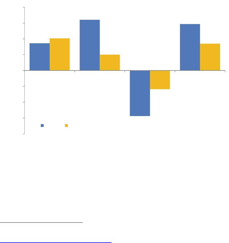
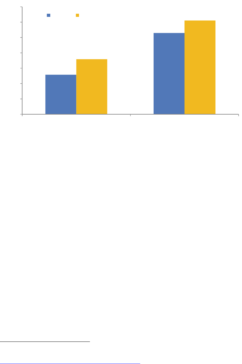
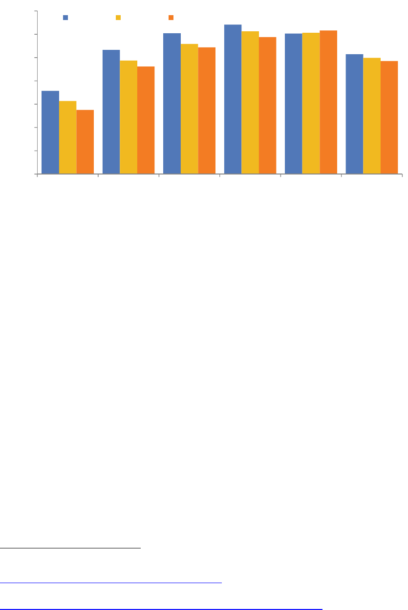
Figure 16 compares the annual net migration estimates over the last three years for the suburban

counties of the Indianapolis metro area, along with the large metros that border the state, against their

average annual levels before the recession. The 10 suburban counties of the Indianapolis metro

averaged a net in-migration of nearly 15,100 residents a year between 2003 and 2007, but this influx

slowed to 6,200 by 2012—a 60 percent decrease.

The net inflow to these same counties jumped to

10,100 last year. Interestingly, the improvement in these counties did not come at the expense of Marion

County, which had a net influx of nearly 2,900 residents in 2013—its best mark in more than two

decades. In all, 62 of Indiana’s 92 counties saw its net migration estimate for 2013 improve over the

previous year.

Figure 16: Comparison of Net Migration Estimates for Suburban Counties of Select Metro

Areas

Source: U.S. Census Bureau population estimates

In the case of the Indianapolis metro area, the suburban counties are Boone, Brown, Hamilton, Hancock, Hendricks, Johnson,

Madison, Morgan, Putnam and Shelby. Marion County is the metro area's core county and is excluded from these numbers.

-20

-10

Chicago Indianapolis Cincinnati Louisville

Net Migration (thousands)

2003 to 2007 Average 2011 2012 2013

As one might expect, improved migration to the state is helping to boost Indiana’s household formation

rate. As Figure 17 shows, after a period of very anemic household growth between 2006 and 2011, the

state’s average household formation rate for the last two years is nearly back to the pre-recession level

seen in the early and mid-2000s. Stated in raw numbers: Indiana added roughly the same number of

households in the last two years (31,300) as it did over the five years between 2006 and 2011 (31,800).

Figure 17: Average Annual Household Formation Rates, 1990 to 2013

Source: U.S. Census Bureau, Decennial Census and American Community Survey

Indiana’s household formation rates could improve even more once the number of households “doubling

up” begins to subside. That is, due to the variety of negative effects associated with the housing crash

and Great Recession, many adults were forced to reside with family or friends. As a result, Indiana’s

headship rate (i.e., the number of households divided by the population age 15 or older), has been on the

decline, particularly among young adults. In 2007, for instance, approximately 50 percent of Hoosiers

between the age of 25 and 34 were the head of their own household, but the headship rate for that same

age group has dropped to 46 percent in 2013. Comparing those same years, age-specific headship rates

are down for each age group with the exception of residents age 65 or older. Therefore, there is a sizable

pool of potentially untapped housing demand in the state that could enter the market as the economy

improves.

Table 3 provides estimates of the shortfall in the number of households in Indiana by age group. The

shortfalls were calculated by looking at the differences in the actual number of households in 2013

compared to the number of households we would expect in 2013 if age-specific headship rates were still

at the levels seen in 2007. The decline in the headship rate for the 25 to 34 age group referenced earlier

translates to more than 31,000 fewer households in the state within this group alone. This number

accounts for 41 percent of the state’s total estimated shortfall. All told, Indiana would have had roughly

77,000 more households in 2013 if headship rates were still at 2007 levels.

1.37%

0.94%

0.62%

0.63%

1.23%

0.69%

0.26%

0.56%

0.0%

0.2%

0.4%

0.6%

0.8%

1.0%

1.2%

1.4%

1.6%

1990 to 2000 2000 to 2006 2006 to 2011 2011 to 2013

Rate of Household Formation

U.S. Indiana

Table 3: Estimated Shortfall in Number of Indiana Households in 2013

Age Group

Actual Number of

Households (thousands)

Number at 2007 Headship

Rates (thousands)

Difference

(thousands)

15 to 24 119.5 136.6 -17.0

25 to 34 386.7 418.2 -31.5

35 to 44 431.2 450.4 -19.2

45 to 54 504.1 518.1 -14.0

55 to 64 480.4 482.9 -2.5

65+ 576.5 568.9 7.6

Total 2,498.4 2,575.0 -76.6

Source: U.S. Census Bureau, American Community Survey

Indiana’s Homeownership Rate Continues to Slide

As new households form in Indiana, will they be looking to buy or rent? If the trend over the past six years

holds, more will be looking to the rental market than was the case before the housing slump. Data from

the Census Bureau’s Housing Vacancy Survey indicate that after a dramatic climb in homeownership

between the mid-1990s and the mid-2000s, the state’s homeownership rate plunged 3 percentage points

between 2008 and 2010. According to the latest decennial census, the state’s homeownership rate stood

at 69.9 percent in 2010, which is below the mark measured in 1990 (70.2 percent) and 2000 (71.4

percent). According to the Census Bureau’s American Community Survey (ACS), the state’s

homeownership rate has continued to slip since 2010, dropping to 68.5 percent in 2013. Indiana ranked

among states in homeownership rate last year.

The focus on the total homeownership rate, however, tends to distract attention from the even larger

declines in most age group-specific rates. Comparing results from the 2000 Census and the 2013 ACS,

for instance, and Indiana’s total homeownership rate was down 2.9 percentage points. The

homeownership rate for Indiana’s 25-to-34 age group, however, is down by 8.2 percentage points over

the same period (see Figure 18). At the same time, the state’s 35-to-44 and 45-to-54 groups are down

7.1 percentage points and 6.1 percentage points, respectively. Only Indiana’s senior age group has seen

its homeownership rate on the rise.

The comparatively small change in the total homeownership rate is simply a function of the fact that the

Indiana population is growing older and the likelihood of being a homeowner increases with age. With the

baby boom generation now between the ages of 50 and 68, this age group holds a larger share of the

state’s population than ever before. This is also the prime age group for homeownership. So the

continued aging of this outsized cohort will boost the state’s total homeownership rate, even if age-

specific rates only hold constant.

Figure 18: Indiana Homeownership Rates by Age, 2000 to 2013

Source: U.S. Census Bureau, Decennial Census and American Community Survey

Looking Ahead

The key demographic drivers for Indiana’s housing market in the next few years will be the direction that

headship rates take and the level of migration to the state. With regard to headship rates, after declining

through the worst of the recession, they have essentially held constant over the last three years in most

age groups. So at worst, the state should not see any further erosion of this measure moving forward. If

Indiana is anything like the nation, however, it should start to see a rebound in headship rates.

Projections from analysts at the Federal Reserve indicate that the U.S. headship rate should improve by

roughly 2 percentage points by the end of this decade.

This increase reflects both the effect of an aging

population and more young adults starting households as the labor market improves.

As for migration, Indiana posted a strong net inflow of residents in 2013 after enduring three years with an

average annual net out-migration. As the economy improves, the state should continue to attract new

residents. The IBRC’s population projections conducted in 2012 indicate that Indiana should expect an

average annual net in-migration of 6,000 residents per year between 2015 and 2020. If Indiana does

continue to see positive net migration and a rebound in headship rates, then household formation should

remain relatively strong, and possibly pick up steam, through the rest of this decade.

As household formation picks up, will age-specific homeownership rates begin to rebound too? Research

indicates that the housing crash has done little to dampen the desire for homeownership among most

Americans, even young adults. According to a Fannie Mae survey conducted in late 2013, 76 percent of

current renters between the ages of 18 and 39 feel that owning a home makes more financial sense than

renting does.

Furthermore, analysis of National Housing Survey data by Harvard researchers shows

Andrew D. Paciorek, “The Long and the Short of Household Formation,” Federal Reserve Board Working Paper, April 2013,

www.federalreserve.gov/pubs/feds/2013/201326/201326pap.pdf.

“What Younger Renters Want and the Financial Constraints They See,” Fannie Mae National Housing Survey, May 2014,

www.fanniemae.com/resources/file/research/housingsurvey/pdf/nhsmay2014presentation.pdf.

20%

30%

40%

50%

60%

70%

80%

90%

25 to 34 35 to 44 45 to 54 55 to 64 65 and older Total

Age Group

2000 2010 2013

that approximately 95 percent of respondents between the ages of 25 and 44 expect to buy a home

sometime in the future.

While the desire to buy a home may be there, the means may not. Seventy-three percent of the younger

renters questioned in the Fannie Mae survey referenced above indicated they believe it would be difficult

for them to get a mortgage, with insufficient credit scores and difficulty saving for a down payment listed

as the top reasons why. Hopefully more and more young adults in this position will be able to access

loans as the labor market improves.

The rate at which younger adults enter the market will be especially important over the next 15 years if

large numbers of retiring baby boomers look to downsize from their current homes. The oldest members

of the baby boom generation turned 65 in 2011 and the entire cohort will be of traditional retirement age

by 2030. According to the IBRC’s population projections, Indiana can expect a slight increase in the

state’s population age 25 to 44 by 2020 (see Figure 19). The 45-to-54 set will decline as the boomers

start to age out of this group and the older brackets will begin their dramatic increase. When the dust

settles in 2030, the share of Indiana’s population that is age 65 or older will increase to 20 percent from

13 percent in 2010.

Figure 19: Indiana Population Projections by Age, 2010 to 2020

Source: Census 2010 and Indiana Business Research Center population projections

This process will impact the housing market in a number of ways, such as increasing demand for senior-

oriented housing. The aging of the baby boomers also has the potential to tilt the balance between

homebuyers and sellers. That is, for the population under the age of 65, the number of homebuyers

typically exceeds the number of sellers, which supports prices and spurs new construction. According to

research from the University of Southern California (USC), this ratio flips around the age of 65, with

Eric S. Belsky, “The Dream Lives On: The Future of Homeownership in America,” Joint Center for Housing Studies, Harvard

University, January 2013, www.jchs.harvard.edu/research/publications/dream-lives-future-homeownership-america.

200

300

400

500

600

700

800

900

1,000

25 to 34 35 to 44 45 to 54 55 to 64 65 to 74 75+

Population (thousands)

2010 2015 2020

sellers outnumbering buyers. The gap between the two begins to widen dramatically after the age of 70.

In most states, this has been manageable because the senior population holds a small share of the total,

but this will change. Over the next 10 years, Indiana’s senior population will boom while the working age

population (i.e., age 25 to 54) is projected to decline slightly.

Because of this dynamic, the USC researchers predict that there is a generational housing bubble on the

horizon.

Their analysis indicates that only six other states (all in the Midwest or Northeast) have a higher

ratio of sellers to buyers in the 65-to-69 age group than Indiana does. If this trend plays out as this study

anticipates, Indiana’s boomers would add more homes to the market without a corresponding increase in

buyers to absorb them. The fact that homeownership rates among younger age groups have declined

only exacerbates this situation. The most likely effect of this shift is that house prices will increase more

slowly in some areas, or maybe even decline, in order to draw more young buyers to the market. This

scenario could also hinder residential construction in some areas.

Some communities will feel the effects of this generational shift more than others will. Fast-growing

suburban counties in the Indianapolis and Louisville metro areas will likely be able to absorb this supply of

homes as younger families continue to move to these communities. Other areas of the state will age more

rapidly, however, as young adults and families move elsewhere. Madison, LaPorte, Howard, Grant and

Wayne counties are examples of larger Indiana communities that could feel the effects of a generational

housing bubble.

Dowell Myers and SungHo Ryu, “Aging Baby Boomers and the Generational Housing Bubble: Foresight and Mitigation of an Epic

Transition,” Journal of the American Planning Association, December 2007.

Housing and the

Economy

Residential Construction Improving, but Still Weak

Residential Fixed Investment (RFI)—a component of GDP that includes investment in new construction

and home improvements—is the most commonly watched indicator of housing’s contribution to the

economy.

One reason that RFI is widely followed is that it tends to be a leading indicator of economic

activity since RFI typically peaks before the start of a recession and it tends to rebound before a downturn

ends, helping to pull the country out of its slump.

However, given housing’s central role in this most

recent economic downturn, RFI is only now beginning to provide much of a boost to the recovery.

While residential investment is beginning to show signs of life, it remains very low by historical standards.

Between 1950 and 2007, RFI accounted for 4.9 percent of annual U.S. GDP on average. As the demand

for new homes nosedived, however, RFI’s share of economic activity bottomed out at 2.5 percent in 2011

and stood at just 3.1 percent in 2013—the fifth-lowest annual mark since the end of World War II. That

said, housing is beginning to make a sustained contribution to economic growth. As of the second quarter

of 2014, RFI has improved for 14 of the past 15 quarters, although it has plateaued at roughly 3.2 percent

of GDP over the last four quarters.

There is no measure of RFI at the state level, but other indicators such as the value of annual building

permits tend to follow the same path. Figure 20 compares the change in national RFI to Indiana’s annual

value of building permits. Both indicators peaked in 2005 and have fallen dramatically since. The total

dollar value of Indiana’s housing permits hit bottom in 2009 and climbed slowly for the next two years

before posting more impressive gains the last couple of years. The value of Indiana’s permits increased

by nearly 31 percent in 2013. Even with this improvement, the value of construction has fallen to an

extent that the dollar total for permits in 2013, even when measured in nominal terms (i.e., not adjusted

for inflation), was a shade below the level seen in 1994.

According to the U.S. Bureau of Economic Analysis, RFI consists of the purchase of residential structures and the residential

equipment that is owned by landlords and rented to tenants. Investment in residential structures includes the new construction of

housing units, improvements to existing housing units, the purchase of manufactured homes and brokers’ commissions on sales.

Kathryn Byun, “The U.S. Housing Bubble and Bust: Impacts on Employment,” Monthly Labor Review, December 2010.

Figure 20: U.S. Residential Fixed Investment and Indiana Value of Building Permits,

1991 to 2013

Source: U.S. Bureau of Economic Analysis and U.S. Census Bureau

The value of housing permits in Indiana continues to rise so far this year, although not at the rate seen

over the last two years. Through July 2014, the total value of permits issued in the state is up 5.6 percent

over the same period in 2013. The harsh weather this past winter and higher mortgage rates may be two

contributing factors to this slowdown.

Housing’s Impact on Employment

The trend in the number of permitted units has been even more dramatic than the value of permits. The

number of units permitted in Indiana in 2013 was only 43 percent of the peak level seen in 1999 and was

the 11th-lowest mark since 1960. However, the number of units last year was up 30 percent over 2012.

One reason for this large increase in residential construction in 2013 was a spike in multi-family

developments. Apartment construction accounted for roughly 30 percent of the new units permitted in

Indiana in 2013—the highest multi-family share since 1986. Nearly 30 percent of the state’s multi-family

units permitted in 2013 were in Hamilton County. Marion and Tippecanoe counties each accounted for an

additional 12 percent of the total.

As with the value of permits, however, the number of new units is growing more slowly this year. Through

July 2014, the number of units is up 6.4 percent over the same period in 2013. Multi-family construction

continues to play a large roll, accounting for 28 percent new units so far this year.

Of course, this lower level of residential construction has triggered a serious decline in employment in this

industry. Compared to 2005, Indiana had nearly 7,600 fewer residential construction jobs in 2013—a 40

percent decline. By comparison, the state’s total employment was off by 1 percent over the same period.

The employment impacts don’t end with the construction industry. With fewer houses built, there is a

reduced demand for other goods and services related to the industry such as architecture and design,

building materials, and home furnishings. According to the IMPLAN economic modeling software,

$100

$200

$300

$400

$500

$600

$700

$800

$900

1991 1993 1995 1997 1999 2001 2003 2005 2007 2009 2011 2013

Indiana Permit Value (billions)

U.S. Residential Fixed Investment

(billions)

U.S. Residential Fixed Investment (left axis)

Indiana Value of Building Permits (right axis)

residential construction has an employment multiplier of 2.1 in Indiana, meaning that each job in this

industry supports an additional 1.1 jobs in other industries throughout the state. If this multiplier holds, the

decline of 7,600 construction jobs between 2005 and 2013 translates to a loss of an estimated 8,360 jobs

in other industries in the state.

Looking Ahead

Clearly, continued improvements in residential construction would be a shot in the arm for the Indiana

economy. Fortunately, several industry forecasts predict that construction activity will remain strong for

the remainder of 2014 and really pick up steam next year. Freddie Mac’s recent forecast, for instance,

predicts that total housing starts in 2014 at the national level will be 10 percent higher than the year

before, and starts in 2015 will be up 28 percent year-over-year. If these forecasts prove to be in the

ballpark, then housing will start to play a larger role in the economic recovery.

Another indication that residential construction may continue to rebound in the next few years is that

vacancy rates continue to decline in Indiana, indicating a tightening housing market. Both the rental

vacancy rate (7 percent) and the homeowner vacancy rate (2 percent) in Indiana have declined to their

lowest levels since at least 2006 (see Figure 21).

Figure 21: Indiana Homeowner and Rental Vacancy Rates, 2006 to 2013

Source: U.S. Census Bureau, American Community Survey

The housing market’s influence on the economy extends beyond construction, however. Most notably,

changes in home values can influence consumer spending. This was especially true during the bubble

era when many homeowners reduced savings in response to what they viewed as permanent and ever-

growing gains in the value of their homes.

Indeed, during the housing bubble, the nation’s personal

“Housing Wealth and Consumer Spending,” Congressional Budget Office, January 2007.

10%

12%

2006 2007 2008 2009 2010 2011 2012 2013

Homeowner Vacancy Rate

Rental Vacancy Rate

Rental Vacancy Rate (left axis)

Homeowner Vacancy Rate (right axis)

savings rate dropped to its lowest levels on record, according to the Bureau of Economic Analysis. This

lower level of savings freed up more money for consumer spending throughout much of the last decade.

The personal savings rate climbed swiftly after the housing bust, but it remains low by historical standards

(the savings rate averaged 10 percent between 1950 and 1998 and has declined sharply of late to a mark

of 5.3 percent in the second quarter of 2014).

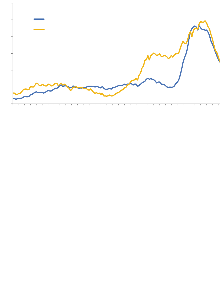
Additionally, during the bubble years, more and more homeowners took advantage of price gains to draw

equity out of their homes through cash-out refinancing (i.e., borrowing more than is needed to pay off the

original mortgage). To demonstrate this trend, data from Freddie Mac shows that homeowners with prime

mortgages cashed out an average of $23 billion in home equity per year between 1993 and 2000. As

Figure 22 shows, this number spiked between 2004 and 2007, averaging $241 billion a year over that

period. At the 2006 peak, cash-out transactions accounted for 87 percent of all refinancing originations.

Figure 22: U.S. Total Home Equity Cashed Out and Personal Savings Rate,

1993:1 to 2014:2

Note: Freddie Mac defines cash-out refinance as a loan amount that is at least 5 percent greater than the unpaid principle balance

of the original loan. The cash-out numbers refer to the refinancing of prime conventional mortgages only. The personal savings rate

numbers are a four-quarter moving average.

Source: Freddie Mac and U.S. Bureau of Economic Analysis

Like the reduced savings rate, the cash-out refinancing boom likely helped to spur some additional

consumer spending. A 2007 Federal Reserve study estimated that homeowners use more than half of

their cashed-out equity on home improvements and other consumer spending.

Also like the reduced

savings rate, this trend proved short-lived. Even as historically low interest rates spurred a surge in

refinancing in 2012 and 2013, cash-out volume as a share of all refinancing over these two years was at

a 20-year low.

Alan Greenspan and James Kennedy, “Sources and Uses of Equity Extracted from Homes,” Federal Reserve Board, March 2007.

$10

$20

$30

$40

$50

$60

$70

$80

$90

1993

1995

1997

1999

2001

2003

2005

2007

2009

2011

2013

Personal Savings Rate

Total Home Equity Cashed Out

(billions)

Total Home Equity Cashed Out (left axis)

Personal Savings Rate (right axis)

Both the decline in personal savings and the increase in cash-out refinancing amounted to more spending

money on hand at a time when real household incomes were stagnant. Given Indiana’s manufacturing

focus—specializing in high-ticket goods like cars, RVs and home furnishings—the state was likely one of

the larger beneficiaries of housing-induced spending. Starting in 2008, however, this spring began to run

dry.

The role of housing wealth as a source of consumer spending will likely never return to bubble-era levels.

For Indiana’s economy to flourish in the next decade, improved income gains here at home and growth in

exports abroad will have to offset this lost demand.

Conclusion

Last year at this time, this report noted that while many phases of the Indiana housing market were

seeing strong improvements, the drivers of housing demand—a strong labor market, migration and

favorable lending conditions—were not yet to a point where they could support sustained growth. It

appears the opposite is the case so far this year, which isn’t such a bad thing. Gains in residential

construction and house prices have moderated so far in 2014 and existing home sales have declined a

bit. Meanwhile, measures of employment growth, unemployment, net migration and household formation

have all moved firmly in the right direction in Indiana, and there are indications that access to mortgage

credit is improving nationally. These developments put Indiana’s housing markets on more solid footing.

While we would have all liked to see double-digit increases in the rate of home sales and construction

continue for a while longer, that level of growth can’t be sustained for long. What the state needs most is

to shore up the economic and demographic foundations of a strong housing market to allow for steady

growth. In the last 12 to 18 months, Indiana has come a couple of steps closer to reaching that goal.

Appendix

Home Sales and Median Sales Price by County, Year-over-Year Change, July

2013 to June 2014

County

Sales, July

2012 to

June 2013

Sales, July

2013 to

June 2014

Percent

Change

Median Price,

July 2012 to

June 2013

Median Price,

July 2013 to

June 2014 Percent Change

Indiana Total 72,458 73,894 2.0% $120,000 $124,000 3.3%

Adams 241 264 9.5% $83,000 $83,250 0.3%

Allen 4,672 4,862 4.1% $112,000 $112,000 0.0%

Bartholomew 977 1,049 7.4% $142,000 $152,000 7.0%

Benton 67 90 34.3% $55,000 $61,000 10.9%

Blackford 93 83 -10.8% $53,500 $54,000 0.9%

Boone 1,040 1,069 2.8% $193,950 $205,000 5.7%

Brown 162 173 6.8% $144,900 $140,000 -3.4%

Carroll 161 162 0.6% $98,450 $88,650 -10.0%

Cass 353 318 -9.9% $63,000 $62,000 -1.6%

Clark 1,450 1,612 11.2% $121,000 $127,000 5.0%

Clay 206 213 3.4% $76,000 $80,000 5.3%

Clinton 205 213 3.9% $80,000 $76,000 -5.0%

Crawford 56 71 26.8% $65,000 $84,000 29.2%

Daviess 201 190 -5.5% $95,000 $81,450 -14.3%

Dearborn 446 490 9.9% $133,940 $140,000 4.5%

Decatur 216 255 18.1% $107,000 $114,500 7.0%

DeKalb 455 450 -1.1% $95,000 $95,000 0.0%

Delaware 987 1,022 3.5% $81,750 $82,500 0.9%

Dubois 404 331 -18.1% $124,800 $124,000 -0.6%

Elkhart 1,744 1,752 0.5% $107,900 $112,000 3.8%

Fayette 148 141 -4.7% $60,000 $61,272 2.1%

Floyd 1,016 1,064 4.7% $135,500 $130,000 -4.1%

Fountain 50 41 -18.0% $86,000 $66,500 -22.7%

Franklin 121 121 0.0% $129,500 $140,000 8.1%

Fulton 164 173 5.5% $72,500 $80,500 11.0%

Gibson 300 306 2.0% $94,900 $99,900 5.3%

Grant 579 564 -2.6% $65,000 $70,000 7.7%

Greene 131 149 13.7% $76,500 $75,900 -0.8%

Hamilton 6,017 6,171 2.6% $197,000 $212,825 8.0%

Hancock 1,056 1,132 7.2% $137,000 $139,350 1.7%

Harrison 342 418 22.2% $127,300 $120,000 -5.7%

Hendricks 2,542 2,621 3.1% $141,000 $152,000 7.8%

Henry 350 331 -5.4% $61,000 $63,000 3.3%

County

Sales, July

2012 to

June 2013

Sales, July

2013 to

June 2014

Percent

Change

Median Price,

July 2012 to

June 2013

Median Price,

July 2013 to

June 2014

Percent Change

Howard 1,074 1,029 -4.2% $77,000 $81,000 5.2%

Huntington 416 403 -3.1% $82,950 $81,500 -1.7%

Jackson 421 383 -9.0% $97,305 $99,500 2.3%

Jasper 287 297 3.5% $133,750 $136,250 1.9%

Jay 75 105 40.0% $55,000 $55,500 0.9%

Jefferson 281 286 1.8% $100,500 $114,400 13.8%

Jennings 120 148 23.3% $87,000 $83,500 -4.0%

Johnson 2,318 2,404 3.7% $127,000 $132,000 3.9%

Knox 244 282 15.6% $79,900 $85,250 6.7%

Kosciusko 889 980 10.2% $128,700 $126,500 -1.7%

Lagrange 278 244 -12.2% $105,000 $114,950 9.5%

Lake 5,026 5,258 4.6% $125,000 $129,900 3.9%

LaPorte 1,072 1,087 1.4% $111,270 $114,000 2.5%

Lawrence 375 407 8.5% $80,000 $85,000 6.3%

Madison 1,441 1,394 -3.3% $81,300 $77,000 -5.3%

Marion 11,481 11,660 1.6% $108,000 $115,000 6.5%

Marshall 366 366 0.0% $112,900 $118,750 5.2%

Martin 30 45 50.0% $92,000 $64,750 -29.6%

Miami 283 276 -2.5% $43,250 $55,000 27.2%

Monroe 1,509 1,473 -2.4% $153,500 $154,500 0.7%

Montgomery 412 455 10.4% $92,000 $97,500 6.0%

Morgan 878 920 4.8% $130,500 $127,000 -2.7%

Newton 124 130 4.8% $97,900 $84,600 -13.6%

Noble 486 438 -9.9% $88,950 $90,000 1.2%

Ohio 39 33 -15.4% $132,500 $100,000 -24.5%

Orange 37 48 29.7% $64,500 $65,000 0.8%

Owen 131 127 -3.1% $79,950 $85,100 6.4%

Parke 51 50 -2.0% $71,450 $70,750 -1.0%

Perry 87 110 26.4% $70,000 $85,000 21.4%

Pike 76 94 23.7% $74,900 $80,000 6.8%

Porter 1,985 2,053 3.4% $166,900 $165,000 -1.1%

Posey 169 193 14.2% $104,950 $102,500 -2.3%

Pulaski 46 52 13.0% $64,010 $84,250 31.6%

Putnam 430 398 -7.4% $109,000 $112,000 2.8%

Randolph 126 152 20.6% $60,000 $54,824 -8.6%

Ripley 221 200 -9.5% $104,900 $115,000 9.6%

Rush 10 10 0.0% $38,500 $15,500 -59.7%

Scott 166 182 9.6% $65,000 $81,200 24.9%

Shelby 524 441 -15.8% $99,900 $111,250 11.4%

Spencer 164 152 -7.3% $116,200 $117,950 1.5%

St. Joseph 2,815 2,638 -6.3% $106,000 $113,725 7.3%

Starke 190 166 -12.6% $76,250 $79,900 4.8%

County

Sales, July

2012 to

June 2013

Sales, July

2013 to

June 2014

Percent

Change

Median Price,

July 2012 to

June 2013

Median Price,

July 2013 to

June 2014

Percent Change

Steuben 488 446 -8.6% $118,000 $127,250 7.8%

Sullivan 105 91 -13.3% $64,000 $78,950 23.4%

Switzerland 49 46 -6.1% $80,000 $98,750 23.4%

Tippecanoe 2,046 2,023 -1.1% $129,000 $133,000 3.1%

Tipton 137 127 -7.3% $79,250 $85,000 7.3%

Union 12 17 41.7% $52,500 $63,000 20.0%

Vanderburgh 2,181 2,264 3.8% $113,500 $112,000 -1.3%

Vermillion 88 118 34.1% $59,950 $52,000 -13.3%

Vigo 996 992 -0.4% $87,400 $84,000 -3.9%

Wabash 262 317 21.0% $65,000 $76,000 16.9%

Warren 43 38 -11.6% $89,500 $73,000 -18.4%

Warrick 849 818 -3.7% $150,000 $156,000 4.0%

Washington 179 205 14.5% $75,000 $76,750 2.3%

Wells 266 284 6.8% $94,000 $97,500 3.7%

White 228 251 10.1% $115,000 $91,400 -20.5%

Whitley 424 387 -8.7% $107,000 $113,000 5.6%

Note: Home sales data are not available for Wayne County.

Source: Indiana Association of Realtors

Number of Units and Value of Residential Building Permits by County, 2012

to 2013

County

Number of

Units,

2012

Number of

Units,

2013

Percent

Change

Value of Permits

(in thousands),

2012

Value of Permits

(in thousands),

2013

Percent

Change

Indiana Total 13,781 17,950 30.3% $2,349,906 $3,065,787 30.5%

Adams 66 56 -15.2% $10,798 $9,226 -14.6%

Allen 1,152 893 -22.5% $168,216 $179,991 7.0%

Bartholomew 200 241 20.5% $45,969 $59,560 29.6%

Benton 1 5 400.0% $592 $2,033 243.4%

Blackford 4 2 -50.0% $363 $592 63.1%

Boone 498 840 68.7% $91,801 $142,972 55.7%

Brown 36 48 33.3% $7,394 $9,288 25.6%

Carroll 0 0 n/a $0 $0 n/a

Cass 9 12 33.3% $1,505 $2,060 36.9%

Clark 499 533 6.8% $67,709 $74,541 10.1%

Clay 15 18 20.0% $1,733 $2,105 21.5%

Clinton 0 28 n/a $0 $5,037 n/a

Crawford 0 0 n/a $0 $0 n/a

Daviess 15 23 53.3% $1,794 $3,055 70.3%

Dearborn 44 68 54.5% $10,057 $14,548 44.7%

Decatur 29 36 24.1% $5,219 $8,719 67.1%

DeKalb 64 79 23.4% $12,023 $14,954 24.4%

Delaware 260 284 9.2% $17,915 $29,030 62.0%

County

Number of

Units,

2012

Number of

Units,

2013

Percent

Change

Value of Permits

(in thousands),

2012

Value of Permits

(in thousands),

2013

Percent

Change

Dubois 84 107 27.4% $10,218 $22,024 115.5%

Elkhart 221 303 37.1% $39,308 $60,976 55.1%

Fayette 4 11 175.0% $725 $1,431 97.4%

Floyd 140 153 9.3% $32,534 $40,055 23.1%

Fountain 6 4 -33.3% $412 $929 125.5%

Franklin 23 35 52.2% $5,082 $6,840 34.6%

Fulton 13 14 7.7% $2,763 $3,135 13.5%

Gibson 56 101 80.4% $9,052 $17,456 92.8%

Grant 36 48 33.3% $5,065 $8,190 61.7%

Hamilton 2,137 3,635 70.1% $479,074 $656,739 37.1%

Hancock 209 327 56.5% $44,018 $50,918 15.7%

Harrison 83 92 10.8% $15,301 $35,807 134.0%

Hendricks 646 1,039 60.8% $117,959 $168,124 42.5%

Henry 16 13 -18.8% $2,535 $2,297 -9.4%

Howard 162 151 -6.8% $18,145 $17,304 -4.6%

Huntington 85 50 -41.2% $9,581 $10,100 5.4%

Jackson 120 170 41.7% $13,638 $20,366 49.3%

Jasper 74 58 -21.6% $13,593 $12,134 -10.7%

Jay 17 22 29.4% $2,646 $2,960 11.9%

Jefferson 46 31 -32.6% $6,290 $3,730 -40.7%

Jennings 37 46 24.3% $3,983 $4,632 16.3%

Johnson 594 698 17.5% $100,879 $135,284 34.1%

Knox 33 48 45.5% $5,104 $7,297 43.0%

Kosciusko 225 262 16.4% $29,239 $35,721 22.2%

LaGrange 122 129 5.7% $14,556 $20,168 38.6%

Lake 819 985 20.3% $164,104 $213,174 29.9%

LaPorte 306 113 -63.1% $34,604 $21,378 -38.2%

Lawrence 11 27 145.5% $1,733 $4,565 163.4%

Madison 68 93 36.8% $14,665 $21,286 45.1%

Marion 604 1,309 116.7% $111,730 $185,524 66.0%

Marshall 50 98 96.0% $11,800 $14,788 25.3%

Martin 2 3 50.0% $110 $297 170.0%

Miami 13 12 -7.7% $2,262 $2,056 -9.1%

Monroe 421 516 22.6% $51,156 $59,208 15.7%

Montgomery 40 47 17.5% $6,489 $8,278 27.6%

Morgan 120 106 -11.7% $18,714 $17,990 -3.9%

Newton 13 21 61.5% $2,357 $4,519 91.7%

Noble 67 82 22.4% $11,127 $13,361 20.1%

Ohio 11 4 -63.6% $1,470 $598 -59.3%

Orange 4 4 0.0% $596 $791 32.7%

Owen 0 0 n/a $0 $0 n/a

Parke 2 25 1,150.0% $261 $3,587 1,274.3%

County

Number of

Units,

2012

Number of

Units,

2013

Percent

Change

Value of Permits

(in thousands),

2012

Value of Permits

(in thousands),

2013

Percent

Change

Perry 23 52 126.1% $2,988 $5,322 78.1%

Pike 19 20 5.3% $3,432 $2,701 -21.3%

Porter 398 469 17.8% $83,628 $121,185 44.9%

Posey 98 45 -54.1% $12,389 $8,152 -34.2%

Pulaski 18 13 -27.8% $3,507 $1,907 -45.6%

Putnam 100 83 -17.0% $12,538 $11,858 -5.4%

Randolph 15 15 0.0% $2,458 $2,458 0.0%

Ripley 79 81 2.5% $11,535 $11,715 1.6%

Rush 11 10 -9.1% $1,858 $1,390 -25.2%

Scott 28 30 7.1% $4,356 $3,919 -10.0%

Shelby 50 66 32.0% $5,999 $8,437 40.6%

Spencer 42 34 -19.0% $8,001 $5,941 -25.7%

St. Joseph 582 422 -27.5% $71,941 $64,678 -10.1%

Starke 45 37 -17.8% $7,502 $6,559 -12.6%

Steuben 107 113 5.6% $23,983 $27,089 13.0%

Sullivan 1 2 100.0% $95 $190 100.0%

Switzerland 49 47 -4.1% $2,855 $2,739 -4.1%

Tippecanoe 542 1,080 99.3% $100,979 $129,670 28.4%

Tipton 15 15 0.0% $2,932 $3,127 6.7%

Union 7 6 -14.3% $670 $1,075 60.4%

Vanderburgh 303 302 -0.3% $32,538 $41,988 29.0%

Vermillion 1 65 6,400.0% $70 $8,770 12,428.6%

Vigo 223 184 -17.5% $25,222 $22,595 -10.4%

Wabash 20 24 20.0% $3,557 $4,240 19.2%

Warren 0 16 n/a $0 $1,768 n/a

Warrick 201 322 60.2% $32,885 $46,837 42.4%

Washington 46 45 -2.2% $7,710 $7,189 -6.8%

Wayne 24 26 8.3% $4,470 $4,961 11.0%

Wells 25 49 96.0% $5,293 $9,495 79.4%

White 24 26 8.3% $5,276 $5,026 -4.7%

Note: Residential permit data are not available for Greene County.

Source: U.S. Census Bureau

Housing Affordability Index Methodology

The housing affordability index is designed to measure the degree to which a “typical” middle income

family can afford the mortgage payments on the typical home. To interpret the index, a value of 100

means that the typical family has just enough income to qualify for an 80 percent mortgage on a median-

priced home. The higher the index, the more affordable the housing.

Calculation of affordability indices is dependent on several published data sources and assumptions. The

primary building block is the median existing house sales price published by the National Association of

Realtors (NAR). The NAR price estimates are available for the nation, Census regions and approximately

132 metropolitan areas. Economy.com estimates home prices for counties and states, in addition to the

metropolitan areas not published by the NAR.

Published median family income data for the United States, regions, states, metropolitan and county

areas are used to determine the income available for a home purchase. Since the Census Bureau

publishes median family income for metropolitan and county areas on a decennial basis, Economy.com

estimates the intercensal years.

The affordability indices use the state-level “effective” interest rates released on an annual basis by the

Federal Housing Finance Board. Effective rates are higher than contract rates because they include fees

and charges (points) amortized over the typical seven-year life of a mortgage.

A 20 percent down payment is assumed, being a standard of the housing industry. This implies a loan

amount of 80 percent of the median sales price. Economy.com assumes a maturity of 30 years.

Economy.com assumes a 25 percent coverage ratio, which is the proportion of minimum qualifying family

income allocated to the monthly payment.

Source: Moody’s Economy.com