/nist2:/usr/nlg/jres103-2/wineland/Pwine.259

Volume 103, Number 3, May–June 1998

Journal of Research of the National Institute of Standards and Technology

[J. Res. Natl. Inst. Stand. Technol. 103, 259 (1998)]

Experimental Issues in Coherent Quantum-State

Manipulation of Trapped Atomic Ions

Volume 103 Number 3 May–June 1998

D. J. Wineland, C. Monroe,

W. M. Itano, D. Leibfried

B. E. King, and D. M. Meekhof

National Institute of Standards and

Technology,

Boulder, CO 80303

Methods for, and limitations to, the genera-

tion of entangled states of trapped atomic

ions are examined. As much as possible,

state manipulations are described in terms

of quantum logic operations since the con-

ditional dynamics implicit in quantum logic

is central to the creation of entanglement.

Keeping with current interest, some experi-

mental issues in the proposal for trapped-

ion quantum computation by J. I. Cirac and

P. Zoller (University of Innsbruck) are dis-

cussed. Several possible decoherence mech-

anisms are examined and what may be the

more important of these are identified.

Some potential applications for entangled

states of trapped-ions which lie outside the

immediate realm of quantum computation

are also discussed.

Key words: coherent control; entangled

states; laser cooling and trapping; quantum

computation; quantum state engineering;

trapped ions.

Accepted: February 4, 1998

Available online: http://www.nist.gov/jres

Contents

1. Introduction ............................... 260

2. Trapped Atomic Ions........................ 261

2.1. Ions Confined in Paul Traps ............. 261

2.2. Ion Motional and Internal Quantum States. . 263

2.2.1. Detection of Internal States ........ 264

2.3. Interaction With Additional Applied

Electromagnetic Fields.................. 265

2.3.1. Single Ion, Single Applied Field,

Single Mode of Motion ........... 265

2.3.2. State Dynamics Including Multiple

Modes of Motion ................ 268

2.3.3. Stimulated-Raman Transitions ...... 269

3. Quantum-State Manipulation.................. 270

3.1. Laser Cooling to the Ground State of

Motion .............................. 270

3.2. Generation of Nonclassical States of

Motion of a Single Ion ................. 272

3.2.1. Population Analysis of Motional

States.......................... 272

3.2.2. Fock State ...................... 272

3.2.3. Coherent States .................. 273

3.2.4. Other Nonclassical States.......... 274

3.3. Quantum Logic ....................... 274

Present address: Universita¨t Innsbruck, Institut fu¨r Experimental

Physik, Austria.

3.4. Entangled States for Spectroscopy ........ 278

4. Decoherence............................... 279

4.1. Motional Decoherence.................. 279

4.1.1. Phase Decoherence Caused by

Unstable Trap Parameters......... 280

4.1.2. Radiative Decoherence ........... 280

4.1.3. Radiative Damping/Heating ....... 280

4.1.4. Injected Noise .................. 282

4.1.5. Motional Excitation From Trap

rfFields....................... 283

4.1.6. Fluctuating Patch Fields .......... 285

4.1.7. Field Emission.................. 286

4.1.8. Mode Cross Coupling From Static

Electric Field Imperfections ....... 286

4.1.9. Collisions With Background Gas . . . 287

4.1.10. Experimental Studies of Heating . . . 289

4.1.11. Experimental Studies of Motional

Decoherence ................... 289

4.2. Internal State Decoherence .............. 290

4.2.1. Radiative Decay ................ 291

4.2.2. Magnetic Field Fluctuations ....... 291

4.2.3. Electric Field Fluctuations ........ 292

4.3 Logic Operation Fidelity and Rotation

Angle Errors.......................... 293

4.3.1 Accumulated Errors ............. 294

4.3.2. Pulse Area and Phase Fluctuations . 296

4.4. Sources of Induced Decoherence ......... 297

259

Volume 103, Number 3, May–June 1998

Journal of Research of the National Institute of Standards and Technology

4.4.1. Applied Field Amplitude and

Timing Fluctuations............... 297

4.4.2. Characterization of Amplitude

and Timing Fluctuations ........... 297

4.4.3. Applied Field Frequency and Phase

Fluctuations ..................... 299

4.4.4. Individual Ion Addressing and

Applied Field Position Sensitivity.... 301

4.4.5. Effects of Ion Motion (Debye-Waller

Factors) ........................ 303

4.4.6. Coupling to Spectator Levels ....... 305

4.4.6.1. Polarization Discrimination

of Internal States .......... 305

4.4.6.2. Spectral Discrimination

of States ................. 306

4.4.6.3. Tailoring of Laser Fields .... 307

4.4.6.4. Spontaneous Emission ...... 308

4.4.7. Mode Cross Coupling During Logic

Operations ...................... 309

5. Variations ................................. 310

5.1. Few Ion Accumulators ................. 310

5.2. Multiplexing With Internal States ......... 311

5.3. High-Z Hyperfine Transitions ............ 311

6. Other Applications.......................... 312

6.1. Quantum Correlations .................. 312

6.2. Simulations........................... 313

6.2.1. Mach-zehnder Boson Interferometer

With Entangled States ............. 314

6.2.2. Squeezed-Spin States.............. 315

6.3. Mass Spectrometry and NMR at the Single

Quantum Level........................ 316

6.4. Quantum State Manipulation of Mesoscopic

Mechanical Resonators ................. 319

7. Summary/Conclusions ....................... 320

8. Appendix A. Entangled States and Atomic

Clocks.................................... 321

9. Appendix B. Master Equation for the Density

Matrix of a Radiatively Damped Harmonic

Oscillator ................................. 322

10. References

............................. 323

1. Introduction

A number of recent theoretical and experimental

papers have investigated the ability to coherently

control or “engineer” atomic, molecular, and optical

quantum states. This theme is manifested in topics such

as atom interferometry, atom optics, the atom laser,

Bose-Einstein condensation, cavity QED, electromag-

netically induced transparency, lasing without inver-

sion, quantum computation, quantum cryptography,

quantum-state engineering, squeezed states, and

wavepacket dynamics. In this paper, we investigate a

subset of these topics which involve the coherent

manipulation of quantum states of trapped atomic ions.

The focus will be on a proposal to implement quantum

logic and quantum computation using trapped ions [1].

However, we will also consider related work on the

generation of nonclassical states of motion and entan-

gled states of trapped ions [2–39]. Many of these ideas

have been summarized in a recent review [40].

Coherent control of spins and internal atomic states

has a long history in NMR and rf /laser spectroscopy.

For example, the ability to realize coherent “

pulses”

or “

/2 pulses” on two-level systems has been routine

for decades. In much of what is discussed in this paper,

we will consider entangling operations, that is, unitary

operations which create entangled states between two or

more separate quantum systems. In particular, we will

be interested in situations where the interaction between

quantum systems can be selectively turned on and off.

For brevity, we will limit discussion to these types of

operations in experiments which involve trapped

atomic ions; however, many of the discussions, in

particular those concerning single trapped ions, will

also apply to trapped neutral atom experiments where

the atoms can be treated as independent. The aspect of

entangling operations is shared by atom optics and atom

interferometry [41, 42] and, as described below, there

are close parallels between the ion trap experiments and

those of cavity QED [43].

Earlier experiments on trapped ions, where the zero-

point of motion was closely approached through laser

cooling, already showed the effects of nonclassical

motion in the absorption spectrum [44–46]. These same

effects can be used to characterize the average energy of

the ion. More recent experiments report the generation

of Fock, squeezed, coherent [21], and Schro¨dinger cat

[47] states. These states appear to be of fundamental

physical interest and possibly of use for sensitive detec-

tion of small forces [26, 48]. For comparison, experi-

ments which detect quantized atomic motion in optical

lattices are reviewed by Jessen and Deutsch [49]. Also,

through the mechanism of Bose-Einstein condensation,

which has recently been observed in neutral atomic

vapors [50–53], a macroscopic occupation of a single

motional state (the ground state of motion) is achieved.

Simple quantum logic experiments have been carried

out with single trapped ions [17]; the emphasis of future

work will be to implement quantum logic on many ions

[1]. The attendant ability to create correlated, or entan-

gled, states of atomic particles appears to be interesting

from the standpoint of quantum measurement [54] and,

for example, for improved signal-to-noise ratio in

spectroscopy of trapped ions (Sec. 3.4).

Therefore, we will be particularly interested in study-

ing the practical limits of applying coherent control

methods to trapped ions for (1) the generation and

analysis of nonclassical states of motion, (2) the imple-

mentation of quantum logic and computation, and (3)

the generation of entangled states which can improve

260

Volume 103, Number 3, May–June 1998

Journal of Research of the National Institute of Standards and Technology

signal-to-noise ratio in spectroscopy. We will briefly

describe the experimental results in these three areas,

but the main purpose of the paper will be to anticipate

and characterize decohering mechanisms which limit

the ability to produce the desired final quantum states in

current and future experiments. This is a particularly

important issue for quantum computation where many

ions (thousands) and coherent operations (billions) may

be required in order for quantum computation to be

generally useful. Here, we generalize the meaning of

decoherence to include any effect which limits the

purity of the desired final states. A fundamental source

of decoherence will be the coupling of the ion’s motion

and internal states to the environment. Also important is

induced decoherence caused by, for example, technical

fluctuations in the applied fields used to implement the

operations. This division between types of decoherence

is arbitrary since both effects can be regarded as

coupling to the environment; however, the division will

provide a useful framework for discussion. As a unify-

ing theme for the paper, we will find it useful to regard,

as much as possible, the quantum manipulations we

discuss in terms of quantum logic. Of course, the subject

of decoherence is much broader than the specific

context discussed here; the reader is referred to more

general discussions such as the papers by Zurek

[55,56,57].

The paper is organized as follows. In the next section,

we briefly discuss ion trapping. In Sec. 3, we consider

in somewhat more detail the three areas of application

enumerated in the previous paragraph. Since cooling of

the ions to their ground state of motion is a prerequisite

to the main applications discussed in the paper, we out-

line methods to accomplish this in the beginning of Sec.

3. Section 4 is the heart of the paper; here, we attempt

to identify the most important sources of decoherence.

Section 5 briefly discusses some variations on proposed

methods for realizing quantum logic in trapped ions.

Section 6 suggests some additional applications of the

ideas discussed in the paper and Sec. 7 provides a brief

summary.

Such a treatment seems warranted in that several lab-

oratories are investigating the use of trapped ions for

quantum logic and related topics; the authors are aware

of related experiments being pursued at IBM, Almaden;

Innsbruck University; Los Alamos National Labora-

tory; Max Planck Institute, Garching; NIST, Boulder;

and Oxford University. This analysis in this paper

necessarily overlaps, but is also intended to complement,

other investigations [58–66] and will, by no means, be

the end of the story. We hope however, that this paper

will stimulate others to do more complete treatments

and consider effects that we have neglected.

2. Trapped Atomic Ions

2.1 Ions Confined in Paul Traps

Due to their net charge, atomic ions can be confined

by particular arrangements of electromagnetic fields.

For studies of ions at low energy, two types of trap are

typically used—the Penning trap, which uses a combi-

nation of static electric and magnetic fields, and the Paul

or rf trap which confines ions primarily through pon-

deromotive forces generated by inhomogeneous oscil-

lating fields. The operation of these traps is discussed in

various reviews (see for example, Refs. [67]–[70]), and

in a recent book by Ghosh [71]. For brevity, we discuss

one trap configuration, the linear Paul trap, which may

be particularly useful in the context of this paper. This

choice however, does not rule out the use of other types

of ion traps for the experiments discussed here.

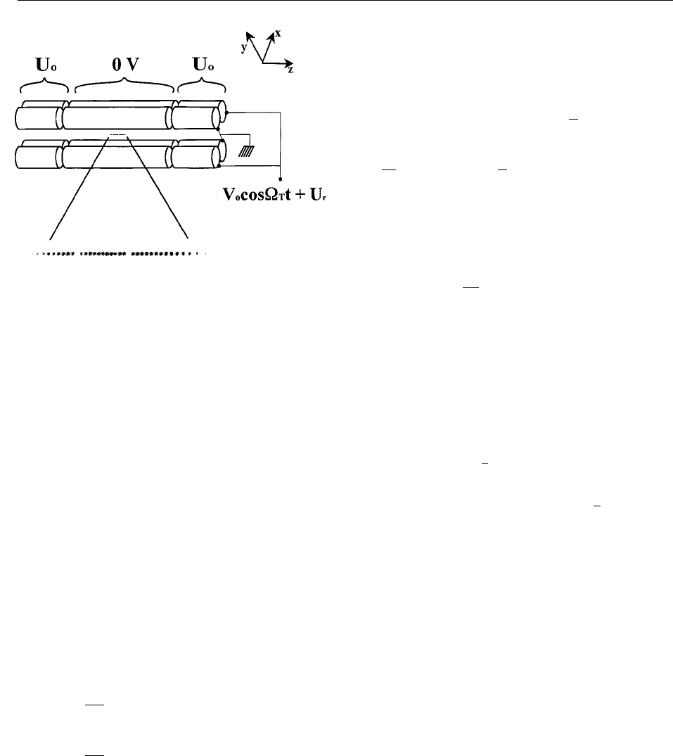
In Fig. 1 we show a schematic diagram of a linear

Paul trap. This trap is based on the one described by

Raizen et al. [72] which is derived from the original

design of Drees and Paul [73]. It is basically a quadru-

pole mass filter which is plugged at the ends with static

electric potentials. A potential V

cos

t + U

is applied

between diagonally opposite rods, which are fixed in a

quadrupolar configuration, as indicated in Fig. 1. We

assume that the rod segments along the z direction are

coupled together with capacitors (not shown) so that the

rf potential is constant as a function of z. Near the axis

of the trap this creates a potential of the form

cos

t + U

)

– y

, (1)

where R is equal to the distance from the axis to the

surface of the electrode. (Unless the rods conform to

equipotentials of Eq. (1), this equation must be multi-

plied by a constant factor on the order of 1; see for

example, Ref. [72].) This gives rise to (harmonic)

ponderomotive potentials in the x and y directions. To

provide confinement along the z direction, static poten-

tials U

are applied to the end segments of the rods as

indicated. Near the center of the trap, this provides a

static harmonic well in the z direction

= kU

–

+ y

)

–

+ y

)

(2)

where k is a geometric factor, m and q are the ion mass

and charge, and

=(2kqU

/m)

1/2

is the oscillation

frequency for a single ion or the center-of-mass (COM)

261

Volume 103, Number 3, May–June 1998

Journal of Research of the National Institute of Standards and Technology

sections, a

(or a) will represent the harmonic oscillator

lowering operator and q

will represent the normal mode

coordinate for the ith mode). The solution of Eqs. (3) to

first order in a

and second order in q

is given by

(t)=A

cos(

t +

)

cos(

cos(2

sin(

t +

) sin(

, (4)

where u

= x or y, A

depends on initial conditions, and

. [a

+ q

/2]

1/2

. (5)

The large amplitude oscillation at frequency

is typi-

cally called the “secular” motion. When a

<< q

<< 1

and U

. 0, if we neglect the micromotion (the terms

which oscillate at

and 2

), the ion behaves as if it

were confined in a harmonic pseudopotential

in the

radial direction given by

+ y

) , (6)

where

. qV

/(2

1/2

)=q

/(2Ï2) is the radial

secular frequency

. For most of the discussions in this

paper, we will assume U

= 0; however it may be useful

in some cases to make U

Þ 0 to break the degeneracy

of the x and y frequencies. Figure 1 also shows an image

of a “string” of

199

ions which are confined near the

z axis of the trap described in Ref. [74]. This was

achieved by making

, thereby forcing the ions

to the axis of the trap. The spacings between individual

ions in this string are governed by a balance of the force

along the z direction due to

and the mutual Coulomb

repulsion of the ions. Example parameters are given in

the figure caption.

When this kind of trap is installed in a high-vacuum

apparatus, ions can be confined for days with minimal

perturbations to their internal structure. Collisions with

background gas can be neglected (Sec. 4.1.9). Even

though the ions interact strongly through their mutual

Coulomb interaction, the fact that the ions are localized

necessarily means that the time-averaged value of the

electric field they experience is zero; therefore electric

field perturbations are small (Sec. 4.2.3). Magnetic field

perturbations to internal structure are important; how-

ever, the coherence time for superposition states of two

internal levels can be very long by operating at fields

Fig. 1. The upper part of the figure shows a schematic diagram of

the electrode configuration for a linear Paul-rf trap (rod spacing .

1 mm). The lower part of the figure shows an image of a string of

199

ions, illuminated with 194 nm radiation, taken with a uv-sensi-

tive, photon counting imaging tube [74]. The spacing between adja-

cent ions is approximately 10 mm. The “gaps” in the string are occu-

pied by impurity ions, most likely other isotopes of Hg

, which do not

fluoresce because the frequencies of their resonant transitions do not

coincide with those of the 194 nm

1/2

→

1/2

transition of

199

oscillation frequency for a collection of identical ions

along the z direction. Equations (1) and (2) represent the

lowest order terms in the expansion of the potentials for

the electrode configuration of Fig. 1. When the size of

the ion sample or amplitude of ion motion is

comparable to the spacing between electrodes or the

spacing between rod segments, higher order terms in

and

become important. However for small oscilla-

tions of the COM mode, which is relevant here, the

harmonic approximation will be valid. In the x and y

directions, the action of the potentials of Eqs. (1) and (2)

gives the (classical) equations of motion described by

the Mathieu equation

+2q

cos(2

)

x =0

+2q

cos(2

)

y = 0, (3)

where

≡

t/2, a

=(4q/m

)(U

– kU

=–(4q/m

)(U

+ kU

), q

=–q

(

). The Mathieu equation can be solved in

general using Floquet solutions. Typically, we will have

< q

<< 1, i [ {x, y}. (Keeping with the usual

notation in the ion-trap literature, in this section, the

symbols a

and q

are defined as above. In all other

262

Volume 103, Number 3, May–June 1998

Journal of Research of the National Institute of Standards and Technology

where the energy separation between levels is at an

extremum with respect to field. For example, in a

(Penning trap) experiment operating in a field of 0.82 T,

a coherence time between hyperfine levels exceeding 10

min was observed [75, 76]. As described below, we will

be interested in coherently exciting the quantized modes

of the ions’ motion in the trap. Here, not surprisingly,

the coupling to the environment is relatively strong be-

cause of the ions’ charge. One measure of the decoher-

ence rate is obtained from the linewidth of observed

motional resonances of the ions; this gives an indication

of dephasing times. For example, the linewidths of

cyclotron resonance excitation in high resolution mass

spectroscopy in Penning traps [77–79] indicate that

these coherence times can be at least as long as several

tens of seconds. Decoherence can also occur from tran-

sitions between the ions’ quantized oscillator levels.

Transition times out of the zero-point motional energy

level have been measured for single

198

ions to be

about 0.15 s [44] and for single

ions to be about

1 ms [45]. These relatively short times are, so far, unex-

plained; however, it might be possible to achieve much

longer times in the future (Sec. 4.1).

In the linear trap, the radial COM vibration frequency

must be made sufficiently higher than the axial COM

vibrational frequency

in order for the ions to be

collinear along the z axis of the trap. This configuration

will aid in addressing individual ions with laser beams

and will also suppress rf heating (Sec. 4.1.5). To prevent

zig-zag and other complicated shapes of the ion crystal,

we require

> 1 for two ions, and

> 1.55 for

three ions. For L > 3 ions, the critical ratio (

)

for

linear confinement has been estimated analytically [80,

81] yielding (

)

. 0.73L

0.86

[60]. Other estimates

are given in Refs. [82] [(

)

. 0.63L

0.865

] and [64]

[(

)

. 0.59L

0.885

]. An equivalent result is obtained

if we consider that as the potential is weakened in the

radial direction, ions in a long string which are spaced

by distance s

near the center of the string, will first

break into a zig zag configuration. At the point where

the ions break into a zig-zag, the net outward force from

neighboring ions is equal to the inward trapping force.

If we equate these forces, we obtain

p«

(3)

, (7)

where

is the Riemann zeta function. As an example,

for

ions, m . 9 u (atomic mass units) and

=3mm, we must have

> 7.8 MHz to keep the

ions along the axis of the trap.

The equilibrium spacing of a linear configuration of

trapped ions is not uniform; the middle ions are spaced

closer than the outlying ions, as is apparent in Fig. 1. The

separation of two ions is s

1/3

s, where

s =(q

)

1/3

is a length scale of ion-ion

spacings; the adjacent separation of three ions is

= (5/4)

1/3

s. For L large, estimates of the minimum

separation of the center ions are given by s

(L)

. 2sL

–0.56

[60], 2.018sL

– 0.559

[61], 2.29L

–0.596

[83], and

1.92sL

– 2/3

[ln(0.8L)]

1/3

[59, 81]. For typical trapping

parameters, the ion-ion separations are on the order of a

few mm and the spatial spread of the zero-point vibra-

tional wavepackets are on the order of 10 nm. Thus there

is negligible wavefunction overlap between ions and

quantum statistics (Bose or Fermi) play no role in the

spatial wavefunction of an array.

Of the 3L normal modes of oscillation in a linear trap,

we are primarily interested in the L modes associated

with axial motion because we will preferentially couple

to them with applied laser fields. A remarkable feature

of the linear ion trap is that the axial mode frequencies

are nearly independent of L[1,60,61,84]. For two ions,

the axial normal mode frequencies are at

and Ï3

;

for three ions they are

, Ï3

, and (5.8)

1/2

. For

L > 3 ions, the Lth axial normal mode can be deter-

mined numerically [60,61,84].

2.2 Ion Motional and Internal Quantum States

A single ion’s motion, or the COM mode of a collec-

tion, has a simple description when the ions are trapped

in a purely static potential, which is the case for the axial

motion in a Penning trap or the axial motion in the trap

of Fig. 1. We will assume that the trap potentials are

quadratic [Eqs. (1) and (2)]. This is a valid approxima-

tion when the amplitudes of motion are small, because

the local potential, expanded about the equilibrium point

of the trap, is quadratic to a good approximation. In this

case, motion is harmonic. An ion trapped in a pondero-

motive potential [Eq. (6)] can be described effectively as

a simple harmonic oscillator, even though the Hamilto-

nian is actually time-dependent, so no stationary states

exist. For practical purposes, the system can be treated

as if the Hamiltonian were that of an ordinary,

time independent harmonic oscillator [34,35,85–91]

although modifications must be made for laser cooling

[92]. The classical micromotion (the terms which vary

as cos

t and cos2

t in Eq. (4)] may be viewed, in the

quantum picture, as causing the ion’s wavefunction to

breathe at the drive frequency

. This breathing mo-

tion is separated spectrally from the secular motion [(at

frequencies

and

in Eq. (4)]. Since the operations

we will consider rely on a resonant interaction at the

secular frequencies, we will average over the compo-

nents of motion at the drive frequency

. Therefore, to

a good approximation, the pseudopotential secular

motion behaves as an oscillator in a static potential.

263

Volume 103, Number 3, May–June 1998

Journal of Research of the National Institute of Standards and Technology

main consequence of the quantum treatment is that

transition rates between quantum levels (Eq. (18),

below) are altered [34, 35]; however, these changes can

be accounted for by experimental calibration. In any

case, for most of the applications discussed in this paper,

we will be considering the motion of the ions along the

axis of a linear Paul trap where this modification is

absent.

Therefore, the Hamiltonian describing motion of a

single ion (or a normal mode, such as the COM mode,

of a collection of ions) in the ith direction is given by

osc

nˆ

, i[{x,y,z} , (8)

where nˆ

≡ a

✝

and a

are the usual harmonic

oscillator raising and lowering operators and we have

suppressed the zero-point energy 1/2

. The operator

for the COM motion in the z direction is given by

z = z

(a + a

✝

) , (9)

where z

/2m

)

1/2

is the spread of the zero-point

wavefunction and m is the ion mass. That is, z

(k0uz

u0l)

1/2

, where unl is the nth eigenstate (“number”

or Fock state) of the harmonic oscillator. For

ions

in a trap where

= 10 MHz, we have z

= 7.5 nm.

Therefore, a general pure state of motion for one mode

can be written, in the Schro¨dinger picture, as

motion

n=0

–n

unl , (10)

where C

are complex and the unl are time-independent.

For applications to quantum logic, we will be interested

in motional states of the simple form

u0l +

exp(– i

t)u1l.

We will be interested in the situation where, at any

given time, we interact with only two internal levels of

an ion. This will be accomplished by insuring that the

internal states are nondegenerate and by using resonant

excitations to couple only two levels at a time. We will

find it convenient to represent a two-level system by its

analogy with a spin-1/2 magnetic moment in a static

magnetic field [93, 94]. In this equivalent representation,

we assume that a (fictitious) magnetic moment

S, where S is the spin operator (S = 1/2), is

placed in a (fictitious) magnetic field

= B

zˆ. The

Hamiltonian can therefore be written

internal

, (11)

where S

is the operator for the z component of the spin

and

≡ –

. Typically, the internal resonant

frequency will be much larger than any motional mode

frequency,

.We label the internal eigenstates

l = u↑l and u↓l representing “spin-up” and “spin-

down” respectively, and for convenience, will assume

< 0 so that the energy of the u↑l state is higher than

the u↓l state. A general pure state of the two-level system

is then given by

internal

= C

↓

u↓l + C

↑

–i

u↑l , (12)

where uC

↓

+ uC

↑

= 1. Of course, the two-level system

really could be a S = 1/2 spin such as a trapped electron

or the ground state of an atomic ion with a single

unpaired outer electron and zero nuclear spin such as

2.2.1 Detection of Internal States

The applications considered below will benefit from

high detection efficiency of the ion’s internal states.

Unit detection efficiency has been achieved in experi-

ments on “quantum jumps” [95–99] where the internal

state of the ion is indicated by light scattering (or lack

thereof), correlated with the ion’s internal state. (More

recently, this type of detection has been used in spec-

troscopy so that the noise is limited by the fundamental

quantum fluctuations in detection of the internal state

[100]. In these experiments, detection is accomplished

with a laser beam appropriately polarized and tuned to

a transition that will scatter many photons if the atom is

in one internal state (a “cycling” transition), but will

scatter essentially no photons if the atom is in the other

internal state. If a modest number of these photons are

detected, the efficiency of our ability to discriminate

between these two states approaches 100 %. We note

that for a string of ions in a linear trap, the scattered light

from one ion will impinge on the other ions; this can

affect the detection efficiency since the scattered light

will, in general, have a different polarization.

The overall efficiency can be explained as follows.

Suppose the atom scatters N total photons if it is

measured to be in state u↓l and no photons if it is mea-

sured to be in state u↑l. In practice N will be limited by

optical pumping but can be 10

or higher [101]. Here,

we assume that N is large enough that we can neglect its

fluctuations from experiment to experiment. We

typically detect only a small fraction of these photons

due to small solid angle collection and small detector

efficiency. Therefore, on average, we detect n

photons where

<< 1 is the net photon detection

efficiency. If we can neglect background, then for each

experiment, if we detect at least one scattered photon,

we can assume the ion is in state u↓l. If we detect

no photons, the probability of a false reading, that is, the

probability the ion is in state u↓l but we simply did not

264

Volume 103, Number 3, May–June 1998

Journal of Research of the National Institute of Standards and Technology

detect any photons, is given by P

(0) =

(1 –

)

. exp(–n

). For n

= 10, P

(0) . 4.5 3 10

–5

for n

= 100, P

(0) . 4 3 10

–44

. Therefore for n

> 10,

detection can be highly efficient.

Detection of ion motion can be accomplished directly

by observing the currents induced in the trap electrodes

[77–79, 102–104]. However, the sensitivity of this

method is limited by electronic detection noise. Because

the detection of internal states can be so efficient, mo-

tional states can be detected by mapping their properties

onto internal states which are then detected (Sec. 3.2).

2.3 Interaction With Additional Applied Electro-

magnetic Fields

2.3.1 Single Ion, Single Applied Field, Single Mode

of Motion

We first consider the situation where a single, period-

ically varying, (classical) electromagnetic field propa-

gating along the z direction is applied to a single trapped

ion which is constrained to move in the z direction in a

harmonic well with frequency

. We consider situa-

tions where fields resonantly drive transitions between

internal or motional states and when they drive transi-

tions between these states simultaneously (entangle-

ment). If we assume that the internal levels

are coupled by electric fields, then the interaction

Hamiltonian is

=–

? E(z, t) , (13)

where

is the electric dipole operator for the internal

transition and E is from a uniform wave propagating

along the z direction and polarized in the x direction,

E = E

xˆcos(kz –

t +

), where

is the frequency, k is

the wavevector 2

,and

is the wavelength. In the

equivalent spin-1/2 analog, we assume that a traveling

wave magnetic field propagates along the z direction, is

polarized in the x direction [B = B

xˆ cos(kz –

t +

)],

and interacts with the fictitious spin (

S).

Therefore, for the spin analog, Eq. (13) is replaced by

=–

? B(z, t)

+ S

–

)(e

i(kz–

)

–i(kz–

)

) , (14)

where

≡ –

/4 (or –

/4 for an electric

dipole), S

≡ S

+ iS

, S

–

≡ S

– iS

and z is given by

Eq. (9). We will assume that the lifetimes of the levels

are long; in this case, the spectrum of the transitions

excited by the traveling wave is well resolved if

sufficiently small.

It will be useful to transform to an interaction picture

where we assume H

= H

internal

+ H

osc

and V

interaction

= H

In this interaction picture, if we make the rotating-wave

approximation (neglecting exp(6i(

)t) terms),

the wavefunction can be written

=↓,↑

n=0

(t)uM

lunl , (15)

where uM

l and unl are the time-independent internal

and motional eigenstates. In general, this wavefunction

will be entangled between the two degrees of freedom;

that is, we will not be able to write the wavefunction as

a product of internal and motional wavefunctions.

We h ave H → H'

= U

✝

(t)H

(t) where U

(t)=

exp(– i(H

)t), resulting in

exp(i[

(ae

–i

+ a

✝

)–

t +

])

+ h.c.(

≡

–

) , (16)

where

≡ kz

is the Lamb-Dicke parameter and

, S

–

, a,anda

✝

are time independent. We will be

primarily interested in resonant transitions, that is,

where

(n' – n) where n' and n are integers. How-

ever, since we want to consider nonideal realizations, we

will assume

=(n' – n)

where u

u <<

.If

we can neglect couplings to other levels (see Sec. 4.4.6),

transitions are coherently driven between levels u↓, n l

and u↑, n' l and the coefficients in Eq. (15) are given by

Schro¨dinger’s equation i

/

t = H'

to be

↑,n'

=–i

(1 + un' – nu)

–i(Dt–

)

n',n

↓,n

=–i

(1 – un' – nu)

i(Dt–

)

n',n

↑,n'

, (17)

where

n',n

is given by [105, 106]

n',n

≡

ukn'u e

(a+a

✝

)

unlu

exp[–

/2](n

!/n

1/2

un'–n|

un'–nu

(

) , (18)

where n

) is the lesser (greater) of n' and n,andL

is the generalized Laguerre polynomial

(X)=

m=0

(–1)

n +

n – m

. (19)

Since we will be particularly interested in small values

of n and

, for convenience, we list a few values of

(X).

265

Volume 103, Number 3, May–June 1998

Journal of Research of the National Institute of Standards and Technology

(X)=1,L

(X)=1–X, L

(X)1–2X +

, L

(X)=1–3X +

–

(X)=1,L

(X)=2–X, L

(X)=3–3X +

, L

(X)=4–6X +2X

–

(X)=1,L

(X)=3–X, L

(X)=6–4X +

, L

(X)=10–10X +

–

(20)

Equations (17) can be solved using Laplace transforms.

The solution shows sinusoidal “Rabi oscillations”

between the states u↑, n'l and u↓, nl, so over the

subspace of these two states we have

(t)=

–i

cos

n',n

+ i

n',n

sin

n',n

–2i

n',n

–i

t–

–

un'–nu

sin

n',n

–2i

n',n

t–

–

un'–nu

sin

n',n

– i

n',n

sin

n',n

+ cos

n',n

(0),

(21)

_ _

where X

n',n

≡ (

n',n

)

1/2

–

–(n' – n)

, and

is given by

= C

↓,n

u↓, nl + C

↑,n'

u↑,n'l =

↑,n'

↓,n

. (22)

For the resonance condition

= 0, Eq. (21) simplifies

(t)=

cos

n',n

–i e

–i[

un'–nu]

sin

n',n

–ie

un'– nu]

sin

n',n

cos

n',n

(0) . (23)

then

<< 1, but the converse is not necessarily true. If

the Lamb-Dicke criterion is satisfied, we can evaluate

n',n

to lowest order in

to obtain

n',n

n,n'

un' – nu

!/n

1/2

(un' – nu!)

–1

. (24)

We will be primarily interested in three types of transi-

tions—the carrier (n' = n), the first red sideband

(n' = n –1), and the first blue sideband (n' = n +1)

whose Rabi frequencies, in the Lamb-Dicke limit, are

given from Eq. (24) by

1/2

, and

(n +1)

1/2

respectively.

In general, the Lamb-Dicke limit is not rigorously

satisfied and higher order terms must be accounted for

in the interaction [16,21,106]. As a simple example,

suppose

(0) = u↓lunl and we apply radiation at

the carrier frequency (

= 0). From Eq. (23), the wave-

function evolves as

When the atom starts in an eigenstate, for each value of

n' – n, the phase factor

un'– nu/2 can be chosen

arbitrarily for the first application of H

; however once

chosen, it must be kept track of if subsequent applica-

tions of H

are performed on the same ion. For conve-

nience, we can choose it to be zero, although in most of

what follows we will include a phase factor as a re-

minder that we must keep track of it. In these expres-

sions, we assume

n',n

to be constant during a given

application time t; this condition can be relaxed as

discussed in Sec. 4.3.2. A special case of interest is

when the Lamb-Dicke criterion, or Lamb-Dicke limit, is

satisfied. Here, the amplitude of the ion’s motion in the

direction of the radiation is much less than

which

corresponds to the condition k

motion

1/2

<< 1. This should not be confused with the less restric-

tive condition where the Lamb-Dicke parameter is less

than 1 (

<< 1); if the Lamb-Dicke criterion is satisfied,

266

Volume 103, Number 3, May–June 1998

Journal of Research of the National Institute of Standards and Technology

(t) = cos

n,n

tu↓, nl – ie

sin

n,n

tu↑, nl . (25)

For n =0,wehave

0,0

exp(–

/2). The exponential

factor in this expression is the Debye-Waller factor

familiar from studies of x-ray scattering in solids; for a

discussion in the context of trapped atoms see Ref. [106]

and Sec. 4.4.5. This factor indicates that the matrix

element for absorption of a photon is reduced due to the

averaging of the electromagnetic wave (averaging of the

ikz

factor in Eq. (14)) over the spread of the atom’s

zero-point wavefunction.

As a second simple example, we consider

(0) = u↓,nl and

(first blue sideband). Equa-

tion (23) implies

(t) = cos

n+1,n

tu↓, nl +e

sin

n +1,n

tu↑, n +1l. (26)

At any time t Þ m

/(2

n+1,n

)(m an integer),

is an

entangled state between the spin and motion. If the

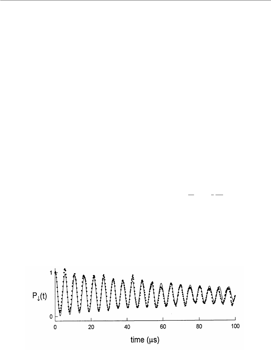
excitation is left on continuously, the atom sinusoidally

oscillates between the state u↓, nl and u↑, n +1l. This

oscillation has been observed in Ref. [21] and is repro-

duced in Fig. 2.

When the Lamb-Dicke confinement criterion is met

and when the radiation is tuned to the red sideband

(

=–

), we find (choosing

=–

/2)

"hV

a + S

–

✝

) . (27)

This Hamiltonian is the same as the “Jaynes-Cummings

Hamiltonian” [107] of cavity QED [43], which

describes the coupling of a two-level atom to a single

mode of the (quantized) radiation field. The problem we

have described here, the coupling of a single two-level

atom to the atom’s (harmonic) motion is entirely

analogous; the difference is that the harmonic oscillator

associated with a single mode of the radiation field in

cavity QED is replaced by that of the atom’s motion.

The suggestion to realize this type of Hamiltonian (in

the context of cavity-QED) with a trapped ion was

outlined in Refs. [2], [3], and [7]; however its use was

already employed in the g-2 single electron experiments

of Dehmelt [108].

Driving transitions between the u↓l and u↑l states will

create entangled states between the internal and

motional states since, in general, the Rabi frequency

will depend on the motional states (Eq. (18)). This

“conditional dynamics,” where the dynamics of one

system is conditioned on the state of another system,

provides the basis for quantum logic (Sec. 3.3).

In this section, we have assumed that the atom inter-

acts with an electromagnetic wave (Eq. (14)), which

will usually be a laser beam. However, the essential

physics which gives rise to entanglement is that the

atom’s internal levels are coupled to its motion through

an inhomogeneous applied field. In the spin-1/2 analog,

the magnetic moment

couples to a magnetic field

B = B(z,t)xˆ , yielding the Hamiltonian

=–

B(z, t)=

–

B(z =0,t)+

B

z

z=0

z +



z

z=0

+...

, (28)

where, as above,

~ S

–

and z is the position

operator. The key term is the gradient



z. From

the atom’s oscillatory motion in the z direction, it expe-

riences, in its rest frame, a modulation of B at frequency

. This oscillating component of B can then drive the

spin-flip transition. As a simple example, suppose B is

static (but inhomogeneous along the z direction so that

Fig. 2. Experimental plot of the probability P

↓

(t) of finding a single

ion in the u↓l state after first preparing

it in the u↓lu0l state and applying the first blue side band coupling (Eq. (16), for

) for a time t. If there

were no decoherence in the system, P

↓

(t) should be a perfect sinusoid as indicated in Eq. (26). Decoherence

causes the signal to decay as discussed in Sec. 3.2.1. The solid line is a fit to an exponentially decaying sinusoid

as indicated in Eq. (43). Each point represents an average of 4000 observations [21].

267

Volume 103, Number 3, May–June 1998

Journal of Research of the National Institute of Standards and Technology



z Þ 0) and

is equal to the resonance frequency

of the internal state transition. In its reference frame,

the atom experiences an oscillating field due to the

motion through the inhomogeneous field. Since

this field resonantly drives transitions between the inter-

nal states. Because this term is resonant, it is the domi-

nant term in Eq. (28), so H

. –

(



z)z ~ (S

–

)(a + a

✝

) . S

a + S

–

✝

, where the last equality ne-

glects nonresonant terms. If the extent of the atom’s

motion is small enough that we need only consider the

first two terms on the right hand side of Eq. (28), H

given by the Janes-Cummings Hamiltonian (Eq. 27)).

This Hamiltonian is also obtained if B is sinusoidally

time varying (frequency

), we satisfy the resonance

condition

–

=–

, and we make the rotating-

wave approximation. This situation was realized in the

classic electron g-2 experiments of Dehmelt, Van Dyck,

and coworkers to couple the spin and cyclotron motion

[108]. Higher-order sidebands are obtained by consider-

ing higher order terms in the expansion of Eq. (28).

One reason to use optical fields is that the field gradi-

ents (for example,



z)[e

ikz

]=ike

ikz

) can be large

because of the smallness of

. Stated another way,

single-photon transitions between levels separated by rf

or microwave transitions, which are driven by plane

waves, may not be of interest because k is small (

large)

and exp(ikz) . 1 which implies



z)[e

ikz

] . 0. This

makes interactions which couple the internal and exter-

nal states as in Eqs. (27) and (28) negligibly small. This

is not a fundamental restriction because electrode struc-

tures whose dimensions are small compared to the wave

length can be used to achieve much stronger gradients

than are achieved with plane waves. Microwave or rf

transitions can also be driven by using stimulated-

Raman transitions as discussed in Sec. 2.3.3 below. A

second reason to use laser fields is they can be focused

so that, to a good approximation, they interact only with

a selected ion in a collection.

The unitary transformations of Eqs. (21) and (23)

form the basic operations upon which most of the

manipulations discussed in this paper are based. In this

section, they were used to describe transitions between

two states labeled u↓lunl and u↑lun'l. In what follows, we

will include other internal states of the atom which will

take on different labels; however, the transitions

between selected individual levels can still be described

by Eqs. (21) and (23). Sequences of these basic opera-

tions can be used to construct more complicated opera-

tions such as logic gates (Sec. 3.3).

2.3.2 State Dynamics Including Multiple Modes of

Motion

In what follows, we will generalize the interaction

with electromagnetic fields to consider motion in all 3L

modes of motion for L trapped ions. Here, as was as-

sumed by Cirac and Zoller [1], we consider that, on any

given operation, the laser beam(s) interacts with only the

jth ion; however, that ion will, in general, have compo-

nents of motion from all modes. In this case Eq. (14) for

the jth ion becomes

+ S

–j

)[e

i(k ? x

–

t +

)

+ h.c.] , (29)

where we now assume k has some arbitrary direction.

We will write the position operator of the jth ion (which

represents the deviation from its equilibrium position)

= u

xˆ+u

L + j

yˆ+u

2L + j

zˆ, j[{1, 2, . . . L} . (30)

We can express the u

in terms of normal mode coordi-

nates q

(k[{1, 2, . . . 3L}) through the matrix D

,by

the following relations [109]

k =1

, q

p =1

, q

≡ q

+ a

✝

(31)

where q

is the operator for the kth normal mode and a

and a

✝

are the lowering and raising operators for the kth

mode. We have assumed that all normal modes are

harmonic, which is a reasonably good assumption as

long as the amplitude of normal mode motion is small

compared to the ion spacing. (For two ions, the axial

stretch mode’s frequency is approximately equal to

(Ï3– 9(a

)

) where a

is the (classical) amplitude

of one ion’s motion for this mode and a

is the ion

spacing). Following the procedure of the last section,

we take H

to be the Hamiltonian of the jth ion’s inter-

nal states and all of the motional (normal) modes

k=1

nˆ

, (32)

where nˆ

≡ a

✝

. In the interaction picture (and making

the rotating wave approximation), we have H'

✝

where U

= exp(– i(H

)t, yielding

exp

k =1

–i

+ a

✝

)–i(dt –

)

+ h.c. , (33)

where

≡ (k ? xˆD

+ k ? yˆ D

L+j

+ k ? zˆD

2L+j

. (For

the linear trap case, motion will be separable in the

268

Volume 103, Number 3, May–June 1998

Journal of Research of the National Institute of Standards and Technology

x, y,andz directions and

will consist of one term.)

In this interaction picture, the wavefunction is given by

= ↓, ↑

}=0

,{n

}

(t)uM

u{n

}l , (34)

where the coefficients are slowly varying and u{n

}l are

the normal mode eigenstates (we have used the short-

hand notation {n

}=n

, n

,...,n

). In analogy with

the previous section, we will be primarily interested in

a particular resonance condition, that is, where

(n'

– n

)and

is sufficiently small that coupling to

other internal levels and motional modes can be ne-

glected. In this case, Eqs. (21) and (23) apply to the

subspace of states u↓l

l and u↑l

un'

l if we make the

definitions

= C

↓,n

u↓l

l + C

↑,n'

u↑l

↑,n'

↓,n

≡

–(n

– n

)

, (35)

and

',n

≡ (

+4(

',n

)

1/2

',n

≡

uk{n

p Þ k

}, n

u P

l=1

+ a

✝

)

u{n

pÞk

}, n

lu.

(36)

The last expression is the Rabi frequency for particular

values of the {n

pÞ k

}. More likely, the other mode states

(pÞ k) will correspond to a statistical distribution; this

is discussed in Sec. 4.4.5. For the application to

quantum logic (Sec. 3.3) the COM mode appears to be

a natural choice since

will be independent of j. The

dependence of

on j for the other modes is not a

fundamental problem, but requires accurate bookkeep-

ing when addressing different ions. The values of

can

be obtained from the normal mode coefficients as

described by James [61].

2.3.3 Stimulated-Raman Transition

As indicated in the discussion following Eq. (28), we

want strong field gradients to couple the internal states

to the motion. If the internal state transition frequency

is small, one way we can achieve strong field gradi-

ents is by using two-photon stimulated-Raman transi-

tions [45, 48] through a third, optical level as indicated

in Fig. 3. In this case, as we outline below, the effective

Hamiltonian corresponding to that in Eq. (14) is

replaced by

+ S

–

)[e

i[(k

– k

) ? x –(

–

)t +

]

+ h.c.] , (37)

where k

, k

and

are the wavevectors and

frequencies of the two laser beams and the resonance

condition between internal states corresponds to

–

u =

. Even if

is small compared to optical

frequencies, uk

– k

u can correspond to the wavevector

of an optical frequency by choosing different directions

for k

and k

; this choice can thereby provide the desired

strong field gradients.

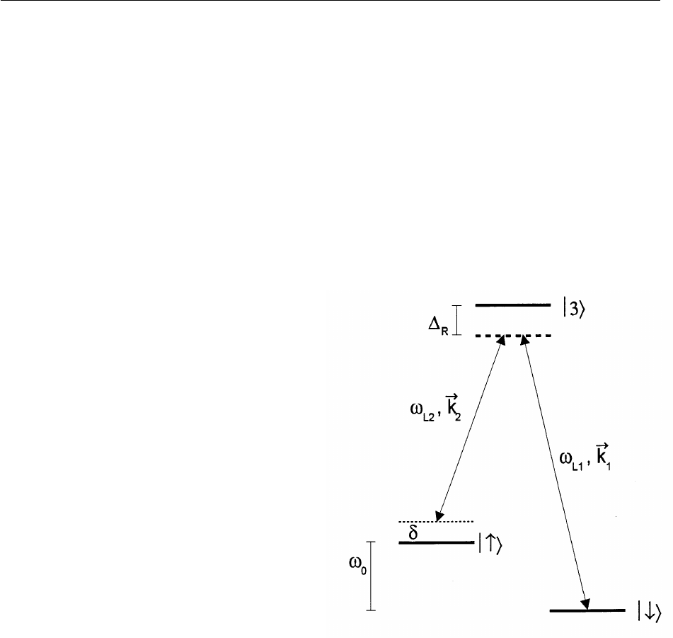
In Fig. 3 we consider that a transition is driven

between states u↓l and u↑l through state u3l by stimu-

lated-Raman transitions using plane waves. Typically,

we consider coupling with electric dipole transitions in

which case

cos(k

? x –

t +

), i[{1, 2} . (38)

For simplicity, we assume laser beam 1 has a cou-

pling only between intermediate state u3l and state u↓l.

Similarly, laser beam 2 has a coupling only between

state u3l and state u↑l. Not shown in Fig. 3 are the

energy levels corresponding to the 3L motional modes.

Laser detunings are indicated in the figure, so

–(

, and we assume

}

where {

} are the 3L mode frequencies. We will

Fig. 3. Schematic diagram relevant to stimulated-Raman transitions

between internal states u↓l and u↑l. Two plane wave radiation fields

couple to a third state u3l. The radiation fields are typically at laser

frequencies; they are characterized by frequencies and wavevectors

and k

, i[{1, 2}. The couplings are typically described by electric

dipole matrix elements. For simplicity, we assume field 1 only cou-

ples states u↓l and u3l; and field 2 only couples states u↑l and u3l.In

this diagram, we do not show the additional energy level structure of

the 3 L modes of motion.

269

Volume 103, Number 3, May–June 1998

Journal of Research of the National Institute of Standards and Technology

assume the Raman beams are focussed so that they

interact only with the jth ion. In the Schro¨dinger picture,

the wavefunction is written

= ↓, ↑,3

}=0

,{n

}

3 exp[– i(

+ n

+... n

)t]

3 uM

u{n

}l , (39)

Since

is large, state u3l can be adiabatically elimi-

nated in a theoretical treatment (see, for example,

Refs. [32], [48], [110], and Sec. 4.4.6.2). If we assume

the difference frequency is tuned to a particular reso-

nance

(n'

– n

), we can neglect rapidly varying

terms and obtain

↑,n

,...n

= i

↑,n

,...n

– i

' , n

↓,n

,...n

↓,n

,...n

= i

↓,n

,...n

– i(

', n

)

↑,n

,...n

(40)

where

≡ –

kn'

+ a

✝

)

l , (41)

where g

≡ E

e k↓u

«ˆ

? ru3l exp(– i

)/(2

≡ E

ek↑u

«ˆ

? ru3lexp(– i

)/(2

≡ (Dk ? xˆD

Dk ? yˆD

L+j

+ Dk ? zˆD

2L + j

and Dk ≡ k

– k

. The

terms ug

and ug

are the optical Stark shifts of

levels u1l and u2l respectively. They can be eliminated

from Eqs. (40) by including them in the definitions of

the energies for the u↓l and u↑l states or, equivalently,

tuning the Raman beam difference frequency

compensate for these shifts. If the Stark shifts are equal,

both the u↓l and u↑l states are shifted by the same

amount, and there is no additional phase shift to be

accounted (Sec. 4.4.3). Equations (40) for stimulated-

Raman transition amplitudes are the same as for the

two-level system (Sec. 2.3.1) if we make the identifica-

tions

–

⇔

and Dk ⇔ k. Although the

experiments can benefit from use of stimulated-Raman

transitions, for simplicity, we will assume single photon

transitions below except where noted.

Another advantage of using stimulated-Raman

transitions on low frequency transitions, as opposed to

single-photon optical transitions, is the difference

frequency between Raman beams can be precisely

controlled using an acousto-optic modulator (AOM) to

generate the two beams from a single laser beam. If the

laser frequency fluctuations are much less than

phase errors on the overall Raman transitions can be

negligible [111]. Other advantages (and some disadvan-

tages) are noted below.

3. Quantum-State Manipulation

3.1 Laser Cooling to the Ground State of Motion

As a starting point for all of the quantum-state manip-

ulations described below, we will need to initialize the

ion(s) in known pure states. Using standard optical

pumping techniques [112], we can prepare the ions in

the u↓l internal state. Laser cooling in the resolved side-

band limit [106, 113 ] can generate the un =0l motional

state with reasonable efficiency [44, 45]. This type of

laser cooling is usually preceded by a stage of

“Doppler” laser cooling [106,114,115] which cools the

ion to an equivalent temperature of about 1 mK. For

Doppler cooling, we have knˆ l $ 1, so an additional stage

of cooling is required.

Resolved sideband laser cooling for a single, harmon-

ically-bound atom can be explained as follows: For sim-

plicity, we assume the atom is confined by a 1-D

harmonic well of vibration frequency

. We use an

optical transition whose radiative linewidth

rad

is rela-

tively narrow,

rad

(Doppler laser cooling applies

when

rad

). If a laser beam (frequency

) is inci-

dent along the direction of the atomic motion, the bound

atom’s absorption spectrum is composed of a “carrier”

at frequency

and resolved frequency-modulation

sidebands that are spaced by

, that is, at frequencies

+(n' – n)

(Sec. 2.3). These sidebands in the spec-

trum are generated from the Doppler effect (like vibra-

tional substructure in a molecular optical spectrum).

Laser cooling can occur if the laser is tuned to a lower

(red) sideband, for example, at

–

. In this case,

photons of energy

(

–

) are absorbed, and sponta-

neously emitted photons of average energy

– R

return the atom to its initial internal state, where R ≡

(

/2m =

is the photon recoil energy of the atom.

Overall, for each scattering event, this reduces

the atom’s kinetic energy by

, a condition

which is satisfied for ions in strong traps. Since

where

is the Lamb-Dicke parameter, this

simple form of sideband cooling requires that the Lamb-

Dicke parameter be small. For example, in

,ifthe

recoil corresponds to spontaneous emission from the

313 nm 2p

1/2

→ 2s

1/2

transition (typically used for

laser cooling),

. 230 kHz. This is to be

270

Volume 103, Number 3, May–June 1998

Journal of Research of the National Institute of Standards and Technology

compared to trap oscillation frequencies in some laser-

cooling experiments of around 10 MHz [45]. Cooling

proceeds until the atom’s mean vibrational quantum

number in the harmonic well is given by

knˆl

min

. (

)

<< 1 [106,115,116].

In experiments, we find it convenient to use two-

photon stimulated Raman transitions for sideband cool-

ing [45, 117], but the basic idea for, and limits to,

cooling are essentially the same as for single-photon

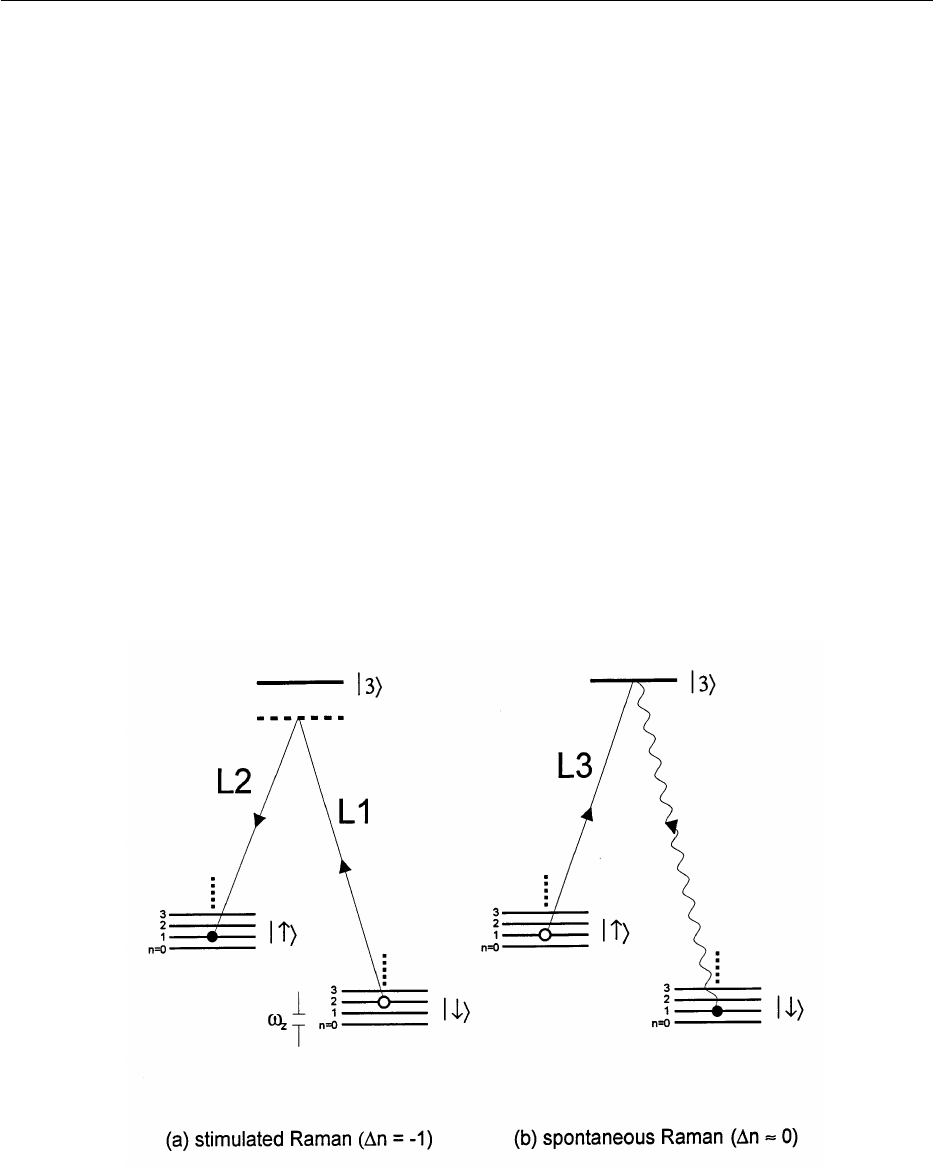
transitions. The steps required for sideband laser cooling

using stimulated-Raman transitions are illustrated in

Fig. 4. This figure is similar to Fig. 3, except we include

the quantum states of the harmonic oscillator for one

mode of motion. Part (a) of this figure shows how, when

the ion starts in the u↓l internal state, a stimulated-

Raman transition tuned to the first red sideband

u↓lunl → u↑lun –1l reduces the motional energy by

. In part (b), the atom is reset to the u↓l internal state

by a spontaneous-Raman transition from a third laser

beam tuned to the u↑l → u3l transition. We assume that

there is a reasonable branching ratio from state u3l to

state u↓l, so that even if the atom decays back to level u↑l

after being excited to level u3l, after a few scattering

events, the atom decays to state u↓l.If

, step (b)

accomplishes the transition u↑lun –1l → u↓lun –1l with

high efficiency. Steps (a) and (b) are repeated until the

atom is optically pumped into the u↓lu 0l state. When this

condition is reached, neither step (a) or (b) is active and

the process stops. In this simple discussion, we have

assumed the transition u↓lunl → u↑lun –1l is accom-

plished with 100% efficiency. However since, in

general, the atom doesn’t start in a given motional state

unl, and since the Rabi frequencies (Eq. (18)) depend on

n, this process is not 100 % efficient; nevertheless, the

atom will still be pumped to the u↓lu0l state. The only

danger is having the stimulated-Raman intensities

and pulse time t adjusted so that for a particular n,

n -1,n

t = m

(m an integer), in which case the atom is

“trapped” in the u↓lunl level. This is avoided by varying

the laser beam intensities from pulse to pulse; one par-

ticular strategy is described in Ref. [17].

So far, laser cooling to the un =0l state has been

achieved only with single ions [44, 45]; therefore an

immediate goal of future work is to laser cool a collec-

tion of ions (or, at least one mode of the collection) to the

zero-point state. Cooling of any of the 3L modes of

motion of a collection of ions should, in principle, work

the same as cooling of a single ion. To cool a particular

mode, we tune the cooling radiation to its first lower

sideband. If we want to cool all modes, sideband cooling

Fig. 4. Schematic diagram relevant to laser cooling using stimulated-Raman transitions. In (a), we

show that when

–

, stimulated-Raman transitions can accomplish the transition u↓l

un l → u↑lun –1l. In the figure, the transition for n = 2 is shown. In (b), spontaneous-Raman transtions,

accomplished with radiation tuned to the u↑l → u3l transition, pumps the atom back to the u↑l state,

thereby realizing the transition u↑lun –1l → u↓lun –1l. When atomic recoil can be neglected, one

application of steps (a) and (b) reduces the atom’s motional energy by

unless n = 0, in which case

the atom is in it’s motional ground state.

271

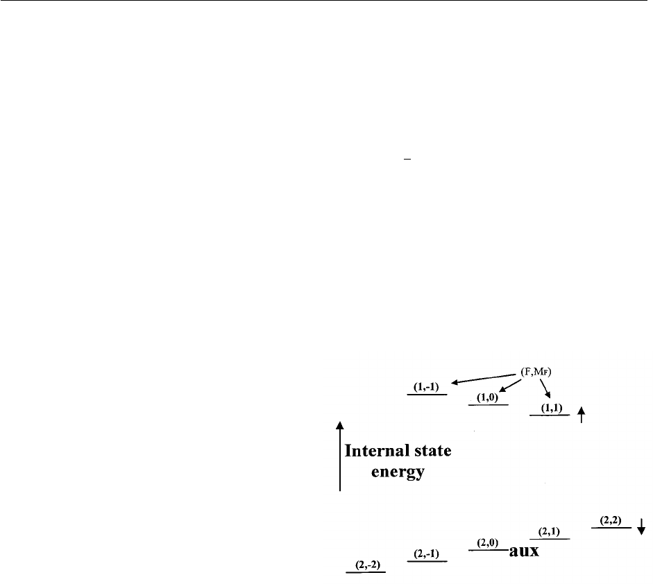
Volume 103, Number 3, May–June 1998

Journal of Research of the National Institute of Standards and Technology

must be cycled through all 3L modes more than once, or

applied to all 3L modes at once, since recoil will heat all

modes. For the COM mode, the cooling is essentially

the same as cooling a single particle of mass Lm;how-

ever, the recoil energy upon re-emission is distributed

over the 3L–1 other modes. Other methods to prepare

atoms in the un =0l state are discussed in Refs. [5], [10],

[12]. Morigi et al. [118] show that it is not necessary to

satisfy the condition

(

<< 1) to achieve

cooling to n =0.

3.2 Generation of Nonclassical States of Motion of

A Single Ion

We begin with a discussion of the generation of non-

classical motional states of a single trapped ion. This

seems appropriate because the other applications

discussed in this paper incorporate similar techniques.

Much of the original interest in nonclassical states

of mechanical motion grew out of the desire to make

sensitive detectors of gravitational waves using (macro-

scopic) mechanical resonators [119, 120]. For example,

parametric amplification of mechanical harmonic oscil-

lations can lead to quantum mechanical squeezing of the

oscillation. In the meantime, nonclassical states of the

radiation field were observed [43]. The close relation-

ship of these two problems was pointed out above: in

quantum optics, H

osc

of Eq. (8) represents a single mode

of the radiation field, and H

of Eq. (14) represents the

coupling between the (quantized) field and atom. The

nonclassical states of motion considered here, such as

squeezed states, are the direct analogs of the nonclassi-

cal photon states in quantum optics. They appear to be

of intrinsic interest because, as in cavity QED, they

allow the rather complicated dynamics of the simple

quantum system [described by the Hamiltonian in

Eq. (27)] to be studied. Before discussing some methods

to create nonclassical states, we consider one method

for analyzing them.

3.2.1 Population Analysis of Motional States

As described below in this section, from the u↓lu0l

state, it is possible to coherently create states of the form

u↓l

motion

where

motion

is given by Eq. (10). One way

we can analyze the motional state created is as follows

[21]: To the state u↓l

motion

, we apply radiation on the

first blue sideband (n'=n + 1 in Eq. (23)) for a time

We then measure the probability P

↓

(

) that the ion is in

the u↓l internal state. In the experiments of Meekhof et

al. [21], the internal state u↓l is the 2s

1/2

(F =2,

= 2) state of

,andu↑l corresponds to the 2s

1/2

(1,1) state as shown in Fig. 5. The u↓l state is detected

by applying nearly resonant

-polarized laser radiation

between the u↓l and

3/2

(F =3,M

= 3) energy levels.

Because the only decay channel of the

3/2

(F =3,

= 3) state is back to the u↓l state, this is a cycling

transition, and detection efficiency is near 1 (Sec. 2.2.1).

The experiment is repeated many times for each value of

, and for a range of

values. We find

↓

(

n =0

–

cos(2

n +1,n

)

, (42)

where P

≡ uC

↓,n

is the probability of finding the ion in

state u↓lunl. The phenomenological decay constants

are introduced to model decoherence that occurs during

the application of the blue sideband. The measured sig-

nal P

↓

(

) can be inverted (Fourier cosine transform),

allowing the extraction of the probability distribution of

vibrational state occupation P

3.2.2 Fock States

In Fig. 2, we show an experimental plot [21] of the

probability P

↓

(

) of finding the ion in the u↓l internal

state after first preparing it in

the u↓lu0l state, and applying the first blue sideband

for a time

. From Eq. (23), we would expect

↓

(

) = cos

1,0

; however, we clearly see the effects

Fig. 5. Hyperfine levels of the 2s

1/2

ground state of

in a weak

magnetic field (not to scale). The energy levels are designated by

horizontal lines. Above the lines, the levels are represented by atomic

physics labels (F, M

) where F is the total angular momentum (elec-

tron plus nuclear angular momentum) and M

is the projection of the

angular momentum along the magnetic field axis. The separation of

Zeeman substates in the different F manifolds is approximately equal

to 0.7 3 10

Hz where B

is expressed is teslas. The separation of

the F = 1 and F = 2 manifolds is approximately 1.25 GHz at B

=0.

For simplicity of notation, in most of the paper we make the identifi-

cations uF =2,M

=2l ≡ u↓l, u1, 1l ≡ u↑l, u2, 0l ≡ uauxl.

272

Volume 103, Number 3, May–June 1998

Journal of Research of the National Institute of Standards and Technology

of some decoherence process which we can represent

adequately by the first term in Eq. (42)

↓

(

1+e

–

cos2

1,0

. (43)

In this experiment, we think the decoherence is not

simply caused by fundamental (radiative) decoherence

but has contributions from fluctuations in laser power

(which cause fluctuations in

1,0

), fluctuations in trap

drive voltage V

(which cause fluctuations in

), and

fluctuations in the ambient magnetic field (which cause

fluctuations in

Neglecting for the moment the effects of decoher-

ence, we see that for times

= m

/(2

1,0

)(m an in-

teger), the ion is in a nonentangled state (u↓lu0l or

u↑lu1l). Therefore, if the ion starts in the u↓lu 0l state, we

can prepare the atom in the u↑lu1l state (the un =1l Fock

state) by applying the blue sideband for a time

1,0

, a so called Rabi

pulse. For other times,

the ion is in an entangled state given by Eq. (26). This

operation and the analogous operation on the first red

sideband will form key elements of quantum logic using

trapped ions.

We can generate higher-n Fock states of motion by a

sequence of similar operations. For example, to generate

the u↓lu2l state, we start in the u↓lu0l state, apply a

pulse on the first blue sideband, followed by a

pulse

on the first red sideband. This leads to the sequence

u↓lu0l → u↑lu1l → u↓lu2l (neglecting overall phase fac-

tors). In a similar fashion, Fock states up to un =16l have

been created [21]. Other methods for creating Fock

states have been suggested in Refs. [5], [8], [12], and

[13].

3.2.3 Coherent States

We can also create coherent states of motion; these

states are closest in character to classical states of mo-

tion. This can be accomplished if the atom is subjected

to a spatially uniform classical force, or any force

derived from a potential – f(t) ? z, where f is a real

c-number vector. For an ion which starts in the un =0l

state, this force creates a displacement leading to a co-

herent state u

l defined by a u

l =

l where

is a

complex number [121]. This classical force can be real-

ized by applying an electric field which oscillates at

frequency

. For example, if we apply a (classical)

electric field E(t)=z

sin(

t–

), the corresponding

interaction Hamiltonian (in the interaction frame for the

motion) is given by

=–qE

(ae

–i

+ a

✝

) sin(

t –

) . (44)

If we express the motional wavefunction as in Eq. (10),

Schro¨dinger’s equation yields for the coefficients of the

wavefunction

ÏnC

n–1

–

Ïn +1C

n +1

, (45)

where

≡ – qE

/(2

). Equivalently, in the inter-

action picture for the motion, the Hamiltonian of Eq.

(44) leads to the evolution operator

U(t)=e

[(

t)a

✝

–(

t)*a]

= D(

t) , (46)

where D is the displacement operator with argument

[121].

We can achieve the same evolution if we superim-

pose two traveling wave fields which drive stimulated-

Raman transitions between different unl levels of the

same internal state, and we make the difference fre-

quency between the Raman beams equal to the trap

oscillation frequency. For example, assume the ion is

subjected to two lasers fields given by Eq. (38), where

–

. The dynamics can be obtained

following the analysis in Sec. 2.3.3, except we replace

level u↓lunl (u↑lun'l) with level uglunl(uglun'l where ugl

can be any ground state which has a matrix element

with level u3l . For the coefficients of Eq. (10), we find

= i

+ ug

–

n'=0

knu

exp[i

(ae

–i

+ a

✝

)–i(

–

)t]+h.c.un'lC

, (47)

where

≡ – g

, g

≡ qE

kgu

«ˆ

? r u3l exp(– i

≡ (k

– k

) ? zˆz

, and

≡

–

. The first

term on the right side of Eq. (47) corresponds to a Stark

shift of level g; this Stark shift can be absorbed into the

definition of the ground state energy (see, for example,

Sec. 4.4.6.2). If this is done, the same equations for the

[Eqs. (47)] are obtained from the Hamiltonian (in the

oscillator interaction picture)

exp

(ae

–i

+ a

✝

)–(

–

)t]

+ h.c. , (48)

In the Lamb-Dicke limit, if we choose the resonance

condition where

–

and assume

Eqs. (47) are the same as Eqs. (45) where

Therefore, in the Lamb-Dicke limit, the applied laser

fields act like a uniform oscillating electric field which

oscillates at frequency

–

. This can be under-

stood if we consider that the two laser fields give rise

to an optical dipole force which is modulated in such

a way to resonantly excite the ion motion. To see

273

Volume 103, Number 3, May–June 1998

Journal of Research of the National Institute of Standards and Technology

this, assume for simplicity that, in Eq. (38), E

= E

«ˆ

,andk

– k

= z

uDku. It is useful to write the

total electric field as

E = E

+ E

ˆ2E(t)

3 cos((k

+ k

) ? z/2 –

t +

) , (49)

where

v¯

≡ (

)/2, f ≡ (

)/2, and E(t)isa

slowly varying function

E(t)=E

cos

z –

–

t +

–

. (50)

On a time scale long compared to 1/

but short com-

pared to 1/(

–

), the atom experiences a nonreso-

nant electric field of amplitude E(t) which is nearly

constant in time. If we consider coupling of this electric

field between the ground state and state u3l (for example,

see Sec. 4.4.6.2), this electric field leads to a spatially-

dependent Stark shift of the ground state equal to

Stark

=–4

ug(z,t)u

where

ug(z,t)u

= ugu

cos

z –

–

t +

–

g ≡

kgu

«ˆ

? ru3le

–i

. (51)

This Stark shift leads to an optical dipole force

122–124] F

=–



(

Stark



z. On a longer time scale,

this dipole force is modulated at frequency

–

which can resonantly excite the ion’s motion when

(

–

. This leads to Eqs. (45). When k

and

are both directed along the z axis (but in opposite

directions), the dipole force potential can be viewed as

a “moving standing wave” in the z direction which slips

over the ion and whose accompanying dipole force reso-

nantly excites the ion’s motion [125]. Both methods

have been used to excite coherent states in Refs. [21] and

[47]. Other methods for generating coherent states are

suggested in Refs. [4] and [48].

In the experiment of Ref. [47], a dipole force oscillat-

ing at the ion oscillation frequency was created with

particular polarizations of the laser fields. This led to a

force which was dependent on the ion’s internal state,

enabling the generation of entangled “Schro¨dinger-cat”

states of the form

=(u↓lu

l + u↑lu

–i

l)/Ï2.

3.2.4 Other Nonclassical States

When (

–

)=2

, a similar analysis shows that

the moving standing wave potential discussed in the last

section has a component which acts like a parametric

excitation of the ion’s harmonic well at frequency 2

[21]. This can produce quantum mechanical squeezing

of the ion’s motion. Squeezing could also be achieved by

amplitude modulating U

at frequency 2

by a nonadi-

abatic change in the trap spring constant [48], or

through a combination of standing and traveling wave

laser fields [4]. A quantum mechanical treatment of the

motion in an rf trap shows the effects of squeezing from

the applied rf trapping fields [34, 35, 91]. More general

nonlinear effects in the interaction can lead to higher

“nonlinear coherent states” as discussed by de Matos

Filho and Vogel [126].

Other methods for generation of Schro¨dinger-cat like

states in ions are suggested in Refs. [8], [19], [29], [31],

[33], [36], and [38]. Additional nonclassical states are

investigated theoretically by Gou and Knight [23], Gou

et al. [37], and Gerry et al. [37]. Schemes which can

generate arbitrary states of the single-mode photon field

[127,128] can also be applied directly to generate

arbitrary motional states of a trapped atom and perform

quantum measurements of an arbitrary motional observ-

able [129]. A scheme which can generate arbitrary

entanglement between the internal and motional levels

of a trapped ion is discussed by Kneer and Law [130].

The procedure for analyzing motional states outlined

in Sec. 3.2.1 yields only the populations of the various

motional states and not the coherences. Coherences

must be verified separately [21, 47]. The most complete

characterization is achieved with a complete state

reconstruction or tomographic technique; a description

of how this has been implemented to measure the

density matrix or Wigner function for trapped atoms is

given in Leibfried et al. [131, 132]. These experiments

represent the first measurement of negative values of the

Wigner function in position-momentum space. Wigner

functions for free atoms have also been recently deter-

mined experimentally by Kurtsiefer et al. [133]. Other

methods for trapped atoms have been suggested in Refs.

[15], [22], [24], [27], [34], and [35]. These techniques

can also be extended to characterize entangled motional

states [39] and states which are entangled between the

motional and internal states.

3.3 Quantum Logic

Significant attention has been given recently to the

possibility of quantum computation. Although this field

is about 15 years old [134–138], interest has intensified

because of the discovery of algorithms, notably for

prime factorization [139–142], which could provide

dramatic speedup over conventional computers.

Quantum computation may also find other applications

274

Volume 103, Number 3, May–June 1998

Journal of Research of the National Institute of Standards and Technology

[142–152]. Schemes for implementing quantum compu-

tation have been proposed by Teich [153], Lloyd [143,

144], Berman et al. [154], DiVincenzo [155, 156], Cirac

and Zoller [1], Barenco et al. [157], Sleator and

Weinfurter [158], Pellizzari et al. [159], Domokos et al.

[160, 161] Turchette et al. [162], Lange et al. [163],

To¨rma¨ and Stenholm [164], Gershenfeld and Chuang

[165], Cory et al. [166], Privman et al. [167], Loss and

DiVincenzo [168], and Bocko et al. [169]. In this paper,

we focus on a scheme suggested by Cirac and Zoller [1],

which uses trapped ions. Since, in general, any quantum

computation can be composed of a series of single-bit

rotations and two-bit controlled-not operations

[140,155,156,170,171], we will focus our attention on

these operations.

In the parlance of quantum computation, we say that

two internal states of an ion can form a quantum bit or

“qubit” whose levels are labeled u0l and u1l or, equiva-

lently, u↓l and u↑l. Single-bit rotations on ion j can be

characterized by the transformation (Eq. (23) for n' = n)

)(C

↓j

u↓l

+ C

↑j

u↑l

)

cos(

/2)

–ie

–i

sin(

/2)

–ie

sin(

/2)

cos(

/2)

↑j

↓j

. (52)

In the spin-1/2 model, this transformation is realized by

application of a magnetic field B

/2 which rotates at

frequency

and in the same sense as

which is

applied slong the direction xˆ cos

– yˆ sin

in the rotat-

ing frame. This is equivalent to application of the field

xˆcos(kz –

t +

) in Eq. (14). In this expression,

n,n

t is the angle of rotation about the axis of

this field. For

and

=0,R(

) is a logical

“not” operation (within an overall phase factor).

/2, –

/2) (plus a rotation about z) is essentially a

Hadamard transform.

A fundamental two-bit gate is a controlled-not (CN)

gate [142,155,156,157]. This provides the transforma-

tion

l → u

l , (53)

where

[{0, 1} and ! is addition modulo 2.

Although Eq. (53) is written in terms of eigenstates, the

transformation is assumed to apply to arbitrary superpo-

sitions of states u

l. In this expression,

is the

called the control bit and

is the target bit. If

=0,the

target bit remains unchanged; if

= 1, the target bit

flips.

A spectroscopy experiment on any four-level quan-

tum system, where the level spacings are unequal, shows

this type of logic structure if we make the appropriate

labeling of the levels. For example, we could label these

four levels as in Eq. (53). If we tune radiation to the

u1, 0l → u1, 1l resonance frequency and adjust its dura-

tion to make a

pulse, we realize the logic of Eq. (53).

Similarly, an eight-level quantum system with unequal

level spacings realizes a Toffoli gate [142], where the

flip of a third bit is conditioned upon the first two bits

being 1’s—and so on (see Sec. 5.2). This basic idea can

be applied to molecules composed of many interacting

spins such as in the proposals of Gershenfeld and

Chuang [165] and Cory et al. [166]. For quantum

computation to be most useful, however, we need to

perform a series of logic operations between an arbi-

trary number of qubits in a system which can be scaled

to large numbers, such as the scheme of Cirac and Zoller

[1].

Another type of fundamental two-bit gate is a phase

gate, which could take the form

l → e

f«

l . (54)

This type of conditional dynamics has been demon-

strated in the context of cavity QED [162,172] and for

a trapped ion [17] (step (1b) below).

The Cirac/Zoller scheme assumes that an array of

ions are confined in a common ion trap. The ions

are held apart from one another by mutual Coulomb

repulsion as shown, for example, in Fig. 1. They can be

individually addressed by focusing laser beams on the

selected ion. Ion motion can be described in terms of

normal modes of oscillation which are shared by all of

the ions; a particularly useful mode might be the COM

axial mode. When quantized, this mode can form the

“bus qubit” through which all gate operations are per-

formed. We first describe how logic is accomplished

between this COM mode qubit and the internal-state

qubit of a single trapped ion. In particular, the transfor-

mation in Eq. (53) has been realized for a single trapped

ion [17]. In that experiment, performed on a trapped

ion, the control bit was the quantized state of one

mode of the ion’s motion (labeled the x mode). If

the motional state was un =0l, this was taken to be a

=0l state; if the motional state was un =1l, this was

taken to be a u

=1l state. The target states were two

ground-hyperfine states of the ion, the uF =2,M

=2l

and uF =1,M

=1l states, labeled u↓l and u↑l

(Fig. 5), with the identification here u↓l ⇔ u

=0l

and u↑l ⇔ u

=1l. Transitions between levels were

275

Volume 103, Number 3, May–June 1998

Journal of Research of the National Institute of Standards and Technology

produced using two laser beams to realize stimulated-

Raman transitions. The wavevector difference k

– k

was chosen to be aligned along the x direction. The CN

operation between these states was realized by applying

three pulses in succession:

(1a) A

/2 pulse (

t =

/4 in Eq. (25), where we

assume

0,0

1,1

) is applied on the carrier

transition. For a certain choice of initial phase,

this corresponds to the operator V

1/2

(

/2) of

Cirac and Zoller [1].

(1b) A 2

pulse is applied on the first blue sideband

transition between levels u↑l and an auxiliary

level uauxl in the ion (the uF =2,M

=0l level in

; see Fig. 5). This operator is analogous to the

operator U

2,1

of Cirac and Zoller [1]. This opera-

tion provides the “conditional dynamics” for the

CN operation. It changes the sign of the u↑l

un =1l component of the wavefunction but leaves

the sign of the u↑lun =0l component of the wave-

function unchanged; that is, the sign change is

conditioned on whether or not the ion is in the

un =0l or un =1l motional state. Therefore, this

step is the phase gate of Eq. (54) with

where we make the identifications (

= 0,1) ⇔

(n = 0,1) and (

= 0,1) ⇔ (internal state = ↓,↑).

(1c) A

/2 pulse is applied to the spin carrier transi-

tion with a 1808 phase shift relative to step (a).

This corresponds to the operator V

1/2

(–

/2) of

Cirac and Zoller [1].

Steps (1a) and (1c) can be regarded as two resonant

pulses (of opposite phase) in the Ramsey separated-field

method of spectroscopy [173]. If step (1b) is active

(thereby changing the sign of the u↑lun =1l component

of the wavefunction), then a state change (spin flip) is

induced by the Ramsey fields. If step (1b) is inactive,

step (1c) reverses the effect of step (1a).

Instead of the three pulses (1a – 1c above), a simpler

CN gate scheme between an ion’s internal and motional

states can be achieved with a single laser pulse, while

eliminating the requirement of the auxiliary internal

electronic level [174], as described below. These simpli-

fications can be important for several reasons:

(1) Several popular ion candidates, including

138

174

172

,and

198

,do

not have a third electronic ground state available

for the auxiliary level. These ions have zero nu-

clear spin with only two Zeeman ground states

= ↓,↑). Although excited optical metastable

states may be suitable for auxiliary levels in some

of these ion species, use of such states places

stringent requirements on the frequency stability

of the exciting optical field to preserve coherence

(see Sec. 4.4.3).

(2) The elimination of an auxiliary ground state level

removes “spectator” internal atomic levels, which

can act as potential “leaks” from the two levels

spanned by the quantum bits (assuming negligible

population in excited electronic metastable

states). This feature may be important to the

success of quantum error-correction schemes

[142, 175–187] which can be degraded when

leaks to spectator states are present [188].

(Specific error-correction schemes for ions are

suggested in Refs. [182] and [187].)

(3) The elimination of the need for an auxiliary level

can dramatically reduce the sensitivity of a CN

quantum logic gate to external magnetic fields

fluctuations. It is generally impossible to find

three atomic ground states whose splittings are all

magnetic field insensitive to first order. However,

for ions possessing hyperfine structure, the tran-

sition frequency between two levels can be made

magnetic field independent to first order at partic-

ular values of an applied magnetic field (see Sec.

4.2.2).

(4) Finally, a reduction of laser pulses simplifies the

tuning procedure and may increase the speed of

the gate. For example, the gate realized in Ref.

[17] required the accurate setting of the phase and

frequency of three laser pulses, and the duration

of the gate was dominated by the transit time

through the auxiliary level.

The CN quantum logic gate can be realized with a single

pulse tuned to the carrier transition which couples the

states unlu↓l and unlu↑l with Rabi frequency

n,n

[see

Eqs. (18), (36), and (41)]. Considering only a single

mode of motion,

n,n

uknue

(a + a

✝

)

unlu =

–

(

) , (55)

where

(

) ≡ L

(

) (Eq. (18)). Specializing to the

un =0l and un =1l vibrational levels relevant to quantum

logic, we have

0,0

–

1,1

–

(1 –

) . (56)

The CN gate can be achieved in a single pulse by

setting

so that V

1,1

0,0

=(2k + 1)/2m, with k and m

positive integers satisfying m > k $ 0. Setting

1,1

0,0

=2m/(2k + 1) will also work, with the roles of the u0l

and u1l motional states switched in Eq. (53). By driving

276

Volume 103, Number 3, May–June 1998

Journal of Research of the National Institute of Standards and Technology

the carrier transition for a duration

such that

1,1

=(k + 1/2)

,ora“

-pulse” (mod 2

)onthe

unl = u1l component, this forces

0,0

= m

. Thus the

states u↓lu1l and u↑lu1l are swapped, while the states

u↓lu0l and u↑lu0l remain unaffected. The net unitary

transformation, in the {↓0, ↑0, ↓1, ↑1} basis is

100 0

010 0

000 ie

(– 1)

k–m

00ie

–i

(–1)

k–m

0 (57)

This transformation is equivalent to the reduced CN of

Eq. (53), apart from phase factors which can be elimi-

nated by the appropriate settings of the phase of subse-

quent logic operations [157].

The “magic” values of the Lamb-Dicke parameter

which allow the above transformation satisfy

(

)=1–

=(2k + 1)/2m, and are tabulated in

Table I of Ref. [174] for the first few values. [For rf

(Paul) trap confinement along the COM motional mode,

the Rabi frequencies of Eqs. (55) and (56) must be

altered to include effects from the micromotion at the rf

drive frequency

. In the pseudopotential approxima-

tion (

), this correction amounts to replacing the

Lamb-Dicke parameter

in this paper by

[1 –

(2Ï2

)], as pointed out by Bardroff et al. [34, 35].

However, there is no correction if the COM motional

mode is confined by static fields (such as the axial COM

mode of a linear trap.)] It may be desirable for the

reduced CN gate to employ the unl = u2l or unl = u3l state

instead of the unl = u1l state for error-correction of

motional state decoherence [182]. In these cases, the

“magic” Lamb-Dicke parameters satisfy

(

1–2

/2=(2k + 1)/2m for quantum logic with

unl = u0l and u2l,or

(

)=1–3

/2 –

/6 =

(2k + 1)/2m for quantum logic with unl = u0l and u3l.

This scheme places a more stringent requirement on

the accuracy of

and

, roughly by a factor of m.In

the two-photon Raman configuration (Sec. 2.3.3), the

Lamb-Dicke parameter

kuz

can be controlled by

both the frequency of the trap (appearing in z

) and by

the geometrical wavevector difference

k of the

two Raman beams. Accurate setting of the Lamb-Dicke

parameter should therefore not be difficult. Both

CN-gate schemes are sensitive to excitation in other

modes as discussed in Sec. 4.4.5.

The CN operations between a motional and internal

state qubit described above can be incorporated to

provide an overall CN operation between two ions in a

collection of L ions. Here, we choose the particular ion

oscillator mode to be a COM mode of the collection.

Specifically, to realize a controlled-not C

c,t

between two

ions c = control bit, t = target bit), we first assume the

COM mode is prepared in the zero-point state. The

initial state of the system is therefore given by

S O

= ↓,↑

...

= ↓, ↑

, M

,...M

3 uM

...uM

u0l . (58)

c,t

can be accomplished with the following steps:

(2a) Apply a

-pulse on the red sideband of ion c.

This accomplishes the mapping (

u↓l

u↑l

)u0l → u↓l

(

u0l +

u1l, and corresponds to

the operator U

1,0

of Cirac and Zoller [1]. We note

that in the NIST experiments [17], we prepare the

state (

u↓l + bu↑l)u0l from the u↓l|0l state using

the carrier transition. We can then implement the

mapping (

u↓l + bu↑l)u0l → u↓l(

u0l +

u1l)by

applying a

-pulse on the red sideband. This is

the “keyboard” operation for preparation of arbi-

trary motional input states for the CN gate of

steps 1a – 1c above. Analogous mapping of inter-

nal state superpositions to motional state super-

positions are reported in Refs. [47], [131], and

[132].

(2b) Apply the CN operation (steps 1a – 1c or, the

single carrier pulse described above) between the

COM motion and ion t.

(2c) Apply the inverse of step (2a).

Overall, C

c,t

provides the unitary transformation (in the

{u↓l

u↓l

, u↓l

u↑l

, u↑l

u↓l

, u↑l

u↑l

} basis)

c,t

1000

0100

0001

0010

(59)

which is the desired logic of Eq. (53). Effectively, C

c,t

works by mapping the internal state of ion c onto the

COM motion, performing a CN between the motion and

ion t, and then mapping the COM state back onto ion c.

The resulting CN between ions c and t is the same as the

CN described by Cirac and Zoller [1], because the oper-

ations V

1/2

(

) and U

1,0

commute.

_ _

277

Volume 103, Number 3, May–June 1998

Journal of Research of the National Institute of Standards and Technology

A third possibility, which also uses only one internal

state transition on each ion, is the following. We employ

two nondegenerate motional modes, which we label

here as 1 and 2. These might be the COM modes in two

different directions. We first map the internal state infor-

mation from two qubits j and k onto the separate

motional modes (which are both initially in the un =0l

un =0l

zero-point state). This can be accomplished as

described in step (2a) above. We then apply a condi-

tional phase gate (Eq. (54) with

) to the two

motional modes. This could be accomplished by driving

transition on a second order red sideband, at

frequency

–

, on a particular (extra) ion “g”

which is initially in the u↓l

state. This ion is not used

to store information; it is only used for this one particu-

lar purpose. This would be followed by operations

which map the motional states back onto the internal

states of ions j and k (like step (2c) above). Overall, this

provides a phase gate (Eq. (54) with f =

) between

ions j and k. To make a CN gate between ions j and k,

we need to precede the above operations with a

pulse on the internal state of ion j (or k) and follow the

above operations with a

/2 pulse on the internal state

of ion j (or k).

In this section, we have assumed that each ion can be

addressed independently. Also, since very many such

operations will be desired for a quantum computer, the

accuracy or fidelity of these operations is of crucial

importance. These issues are confronted in Sec. 4. As

noted in Sec. 2.3, in each separate operation involved in

a quantum computation, such as application of the red

sideband in step 2(a) to ion j, a definite phase of the

applied fields is assumed. This phase for each ion can be

chosen arbitrarily for the first operation, but upon

successive applications of the same operation to the

same ion, it must be held fixed, or at least be known,

relative to the initial phase. An exception to this is appli-

cation of 2

-pulses as in step 1(b) where the phase of

the fields does not enter into the final result of the

operation.

3.4 Entangled States for Spectroscopy

A collection of atoms, whose internal states are entan-

gled through the use of quantum logic, can improve the

quantum-limited signal-to-noise ratio in spectroscopy.

Compared to the factorization problem, this application

has the advantage of being useful with a relatively small

number of ions and logic operations. For example, for

high-accuracy, ion-based frequency standards [74,189,

190,191], use of a relatively small number of trapped

ions (L # 100) appears optimum. As outlined here, the

states involving L ions which are useful for spectroscopy

and frequency standards can be generated with L logic

gates. For L . 100, a significant improvement in perfor-

mance in atomic clocks could be expected.

In spectroscopy experiments on L atoms, in which the

signal relies on detecting changes in atomic populations,

we can view the problem in the following way using the

spin-1/2 analog for two-level atoms. The total angular

momentum of the system is given by J =

i=1

where S

is the spin of the ith atom. The basic task is to measure

, the frequency of transitions between the u↓l and u↑l

states Eq. (11). We first prepare an initial state for the

spins. We assume spectroscopy is performed by apply-

ing (classical) fields of frequency

for a time T

according to the method of separated fields by Ramsey

[173]. The same field is applied to all atoms. After

applying these fields, we measure the final state popula-

tions; that is, we detect, for example, the number of

atoms N

↓

in the u↓l state. In the spin-1/2 analog, this

is equivalent to measuring the operator J

, since

↓

= J

–J

where

is the identity operator. We assume

the internal states can be detected with 100 % efficiency

(Sec. 2.2.1). If all sources of technical noise are elimi-

nated, the signal-to-noise ratio (for repeated measure-

ments) is fundamentally limited by the quantum fluctua-

tions in the number of atoms which are observed to be

in the u↓l state. These fluctuations can be called quan-

tum projection noise [100]. Spectroscopy is typically

performed on L initially nonentangled atoms (for exam-

ple,

(t =0)=P

i=1

u↓l

). With the application of the

Ramsey fields, the atoms remain nonentangled. For this

case, the imprecision in a determination of the fre-

quency of the transition is limited by projection noise to

)

meas

= 1/(LT

)

1/2

where t >> T

is the total averag-

ing time [100]. If the atoms can be initially prepared in

particular entangled states, it is possible to achieve

)

meas

< 1/(LT

)

1/2

. Initial theoretical investigations

for ions [3, 9] examined the use of correlated states

which could achieve (D

)

meas

< 1/(LT

)

1/2

when the

population (J

) was measured. These states are

analogous to those previously considered for interferom-

eters [192, 193]. More recent theoretical investigations

[194] consider the initial state to be one where, after the

first Ramsey pulse, the internal state is the maximally

entangled state

Ï2

(u↓l

u↓l

... u↓l

(t)

u↑l

...u↑l

(60)

where

(t)=

– L

t. After applying the Ramsey

fields, we measure the operator O

= P

i=1

instead of

. This gives (D

)

meas

= 1/(L

)

1/2

, which is the max-

imum signal-to-noise ratio possible and corresponds to

the Heisenberg limit [194]. In the language of quantum

––

278

Volume 103, Number 3, May–June 1998

Journal of Research of the National Institute of Standards and Technology

error correction, if we express

in terms of the basis

states u0l' =(u0l + u1l)/2

1/2

and u1l' =(u0l – u1l)/2

1/2

,we

find that

(t) is determined from a parity check of the

total state in this second basis [142]. For an atomic clock

where the interrogation time T

is fixed by other con-

straints, this means that the time

required to reach a

certain measurement precision is reduced by a factor of

L relative to the nonentangled atom case. This improve-

ment is of significant practical importance since, to

achieve high measurement precision, atomic clocks are

run for averaging times

of weeks, months, and even

longer.

Cirac and Zoller [1] have outlined a scheme for pro-

ducing the state in Eq. (60) using quantum logic gates.

Starting with the state

(t =0)=P

i=1

u↓l

u0l,wefirst

apply a

/2 rotation (

0,0

t =

/4,

/2 in Eq. (23))

to ion 1 to create the state

–1/2

(u↓l

+ u↑l

)u↓l

u↓l

...u↓l

u0l. We then apply the CN gate C

1,i

, sequentially

between ion 1 and ions i = 2 through L to achieve the

state of Eq. (60). An alternative method for generating

this state is described in Ref. [194]. As a final example,

we consider a method for generating the maximally

entangled state which requires a fixed number of steps,

independent of the number of ions. For simplicity, we

illustrate the method for three ions. Starting with the

state

(t =0)=u↓lu↓lu↓lu0l, we first selectively drive

one of the ions (say ion 3) with a carrier

/2 pulse

followed by a red sideband

pulse to give the sequence

u↓lu↓lu↓lu0l → 2

–1/2

u↓lu↓l(u↓l + u↑l) u0l → 2

–1/2

u↓lu↓l

u↓l(u0)l + u1l). We now use the Lamb-Dicke dependence

of the carrier transition (Eqs. (56)) to make an odd

(even) integer number of

flips correlated with the

un =0l state and an even (odd) integer number of

flips

correlated with the un =1l state (the laser beam intensity

is assumed to be the same on all ions). We can now

employ a transition to an auxiliary level. For example, if

the state after the last step, is the state 2

–1/2

( u↑lu↑lu↑lu1l

+ u↓lu↓lu↓lu0l), we could apply a blue sideband

pulse

between states u↑l and uauxl of one of the ions (say the

third) followed by a carrier

pulse on this transition to

carry out the steps 2

–1/2

(u↑lu↑lu↑lu1l + u↓lu↓lu↓lu0l) →

–1/2

(u↑lu↑luauxl + u↓lu↓lu↓l)u0l) → 2

–1/2

(u↑lu↑lu↑l +

u↓lu↓lu↓l)u0l. (If the state after the previous step was

–1/2

(u↑lu↑lu↑lu0l + u↓lu↓lu↓lu1l), we would sandwich

the last operation between

pulses on the u↓l → u↑l

transition of the selected ion.)

Other correlated states can also be useful for spec-

troscopy. A strategy which essentially measures the

variance of N

↓

is discussed by Holland and Burnett

[195] and Kim et al. [196]. This method has also been

incorporated into a proposed technique for spectroscopy

of internal states of Bose-Einstein condensates [197].

In comparing the case for entangled vs non-entangled

states in spectroscopy, the above discussion has assumed

that T

is fixed. This constraint would be valid if the ions

were subject to a constant heating rate and we desired to

maintain the second-order-Doppler (time dilation) shift

below a certain value, for example. However, the use of

entangled states may not be advantageous, given other

conditions. For example, Huelga et al. [198] assume that

the ions are subject to a certain dephasing decoherence

rate (decoherence time less than the total observation

time). In this case, there is little advantage of using

maximally entangled states over non-entangled states.

The basic reason is that the maximally entangled state

decoheres L times faster than the states of individual

atoms. Therefore, when using the maximally entangled

state, T

must be reduced by a factor of L for optimum

performance. Because of this, the gain from use of the

maximally entangled state is offset by the reduced value

of T

. (Huelga et al. [198] actually show that a modest

improvement can be obtained under these conditions by

use of partially entangled states.) In appendix A, we

compare entangled vs nonentangled states in the context

of a practical atomic clock application where a refer-

ence oscillator is locked to the atomic resonance.

4. Decoherence

The atomic motional and internal states, and the

(logic) operations, were described above in an idealized

fashion. In this section we consider some of the practical

limitations to these idealizations. These limitations can

generally be grouped under the heading of decoherence

if, by decoherence, we mean any effect which limits the

fidelity of these operations (see Sec. 4.3). This is a more

general use of the term decoherence; in some treat-

ments, decoherence refers only to dephasing of qubit

states and does not include state changes. Although

somewhat arbitrary, we also find it convenient to break

decoherence into categories: (1) decoherence of the ion

motion, (2) decoherence of the ion internal levels, and

(3) decoherence caused by nonideal applied fields

which are responsible for the logic operations.

4.1 Motional Decoherence

For the trapped ion system discussed in this paper,

decoherence may be dominated by that of the motional

state. Scaling of decoherence will depend on the physi-

cal system being treated and the mechanism of decoher-

ence [199, 200]. For quantum computation with ions,

motional decoherence is somewhat easier to character-

ize than for a general motional state since we are

primarily interested in relaxation of the un =0l and

un =1l motional states for a particular mode (for exam-

ple, the center-of-mass (COM) mode along the axis of a

linear trap).

279

Volume 103, Number 3, May–June 1998

Journal of Research of the National Institute of Standards and Technology

4.1.1 Phase Decoherence Caused by Unstable Trap

Parameters

A simple form of motional decoherence is caused by

fluctuations in trap parameters. Most likely, by employ-

ing electronic filtering, these parameters fluctuate

slowly on the time scale of the basic operations

(. 1/

n',n

), therefore, the motion is subject to dephasing

due to the corresponding adiabatic changes in motional

frequency. In the linear trap, if we assume a

<< q

i[{x, y} (Sec. 2.1), then for small fluctuations

,and

R,wehave

x,y

– d

–2dR /R,

= 1/2(d

+ dU

) . (61)

The relationship between these frequency fluctuations

and phase fluctuations in a series of logic operations is

discussed in Sec. 4.3.2. The effects of modulation of

these parameters by high-frequency noise is considered

in Sec. 4.1.3 and in Ref. [66]. Although an experimen-

tally open question, it is expected that all of these

parameters could be controlled sufficiently well that

they should not be the primary cause of decoherence.

4.1.2 Radiative Decoherence

Decoherence has received considerable attention in

connection with quantum measurement [201] and has

been put forth as a practical solution to the quantum

measurement problem [55,56,57]. In quantum optics, a

paradigm for decoherence has been to consider relax-

ation of the harmonic oscillator associated with a single

mode of the radiation field by coupling to the environ-

ment [202–206]. This kind of fundamental decoherence

has recently been observed in the context of cavity QED

by Brune et al. [207]. An important result from these

studies is that relaxation of superposition states occurs at

a rate which increases with the separation of the states

in Hilbert space and almost always precludes the exis-

tence of “large” Schro¨dinger-cat-like states except on

extremely short time scales.

A fundamental source of decoherence for the COM

mode of ion motion is understood by considering that

the dipole associated with the oscillating charged ion(s)

is radiatively coupled to the thermal fields of the envi-

ronment, at temperature T. The master equation describ-

ing the evolution of the density operator

for the motion

(in the interaction picture) can be written [208,209,210]

Ù =

(n¯ + 1) (2a

✝

– a

✝

–

✝

n¯(2a

✝

a – aa

✝

–

✝

) , (62)

where n¯ is the mean number of motional quanta when

the ion is in equilibrium with the environment

(n¯ = [exp(

T)–1]

–1

), and

is the relaxation rate of

the energy to thermal equilibrium. Since ion trap exper-

iments will typically operate in the situation where

<< k

T, then n¯ . k

. We will assume the

ion(s) start in the subspace of density matrix elements

,and

where

≡ ki|

ujl. Equation (62)

implies

(t =0)= Ï2

(n¯+1)

–

(2n¯ + 1/2)

. –2n¯

=–

[n¯

–(n¯+1)

(n¯+1)

–

(3n¯+1)

n¯

. (63)

General expressions for d

/dt and dknˆl/dt are given in

Appendix B. Based on these expressions and in the limit

that n¯ >> 1, we will characterize the motional decoher-

ence by the time t* = 1/(n¯

), which is approximately the

time for the ion to make a transition from the ground

state. This agrees with a classical estimate [103].

4.1.3 Radiative Damping/Heating

The electric dipole associated with the an ion’s COM

oscillatory motion will couple to thermal (black body)

or ambient radiation in the environment. However, since

the wavelength corresponding to ion oscillation frequen-

cies will typically be much larger than the trap electrode

spacings, this coupling can be described by lumped-cir-

cuit models [102, 103]. In these models, we assume the

ion’s motion induces currents in the neighboring elec-

trodes; these currents, in turn, couple to the resistance of

the electrodes or circuit elements attached to the elec-

trodes. In experiments where these resistances are pur-

posely made high to maximize damping of the ion COM

motion, observed time constants agree with the model

[77,78,79,102,103,104]. In the two (single-ion) experi-

ments which have been able to achieve cooling to the

n = 0 motional state, the measured value of t* was about

0.15 s for a

198

ion [44] and about 1 ms for a single

ion [17,21,45,47,131,132,211]. In these experi-

ments, t* was intended to be made as long as possible;

however, the observed values of t* were considerably

shorter than what we would calculate from the model,

as shown below.

The model considers the electric-circuit equivalent

shown in Fig. 6(a). Effectively, the electric-dipole

oscillator formed by the ion COM motion can be consid-

ered to be confined in a cavity formed by the trap

electrodes. A useful representation of this situation is to

model the COM motion (in one direction) as a series

inductive-capacitive (lc) circuit which is shunted by the

280

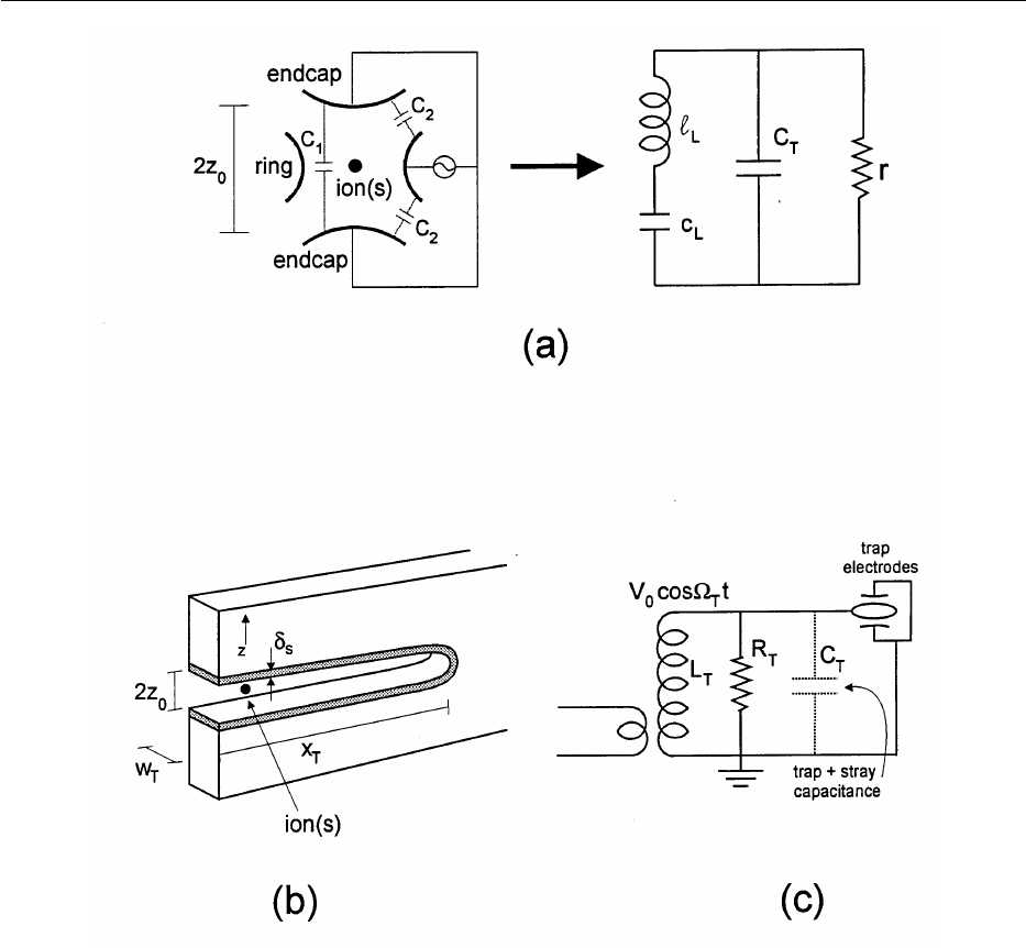
Volume 103, Number 3, May–June 1998

Journal of Research of the National Institute of Standards and Technology

Fig. 6. Schematic diagrams of the lumped circuit equivalents for the trap electrodes and trapped ion(s). (a) The

left part of the diagram shows, schematically, the electrodes for a Paul trap with hyperbolic electrodes and a

collection of trapped ions. On the right is shown the corresponding lumped circuit equivalent; C

represents the

inter-electrode capacitance (the combined effects of the capacitances shown in the left part of the figure); r

represents the resistive losses in the electrodes and connecting wires, l

and c

represent the equivalent inductance

and capacitance for the COM mode of oscillation in the z (vertical) direction [103]. (b) A schematic diagram of

the endcaps electrode for the trap of Jefferts et al. [211] which was used in the NIST experiments (the ring is

not shown). Induced currents in the z (vertical) direction are assumed to follow a path indicated by shading; the

resistance in this path represents r in part (a) of the figure. (c) The rf potential between ring and endcaps electrode

(or between pairs of rods as indicated in Fig. 1) is typically generated with a resonant rf step-up transformer. The

resistance in this transformer can, in principle, couple to the ion motion as discussed in the text.

capacitance of the trap electrodes as shown [9, 103].

The resistance r is due to losses in the electrodes and

conductors which connect the electrodes. The Johnson

noise associated with this resistance can heat the ions.

The equivalent inductance of the ion COM motion is

given by l

. md

/L(

where d is the characteristic

internal dimension of the ion trap electrodes, L the num-

ber of ions, and

is a geometrical factor on the order of

1 which can be computed [212]. For traps with hyper-

bolic electrodes, if we consider motion in the z direc-

tion, d =2z

(the separation of the endcap electrodes)

[67–70] and

. 0.8 [213,214,215]. For the trap used in

the NIST experiments, where z

= 130 mm, l

. 60 000

henries! The resistance r yields a time constant

/r =1/

. This implies [9]

281

Volume 103, Number 3, May–June 1998

Journal of Research of the National Institute of Standards and Technology

n¯

(

)

, (64)

where Q =

/r is the quality factor of the ion oscilla-

tor. The last expression in Eq. (64) shows t* in terms of

the spectral density of electric field fluctuations at the

site of the ion which can be written S

=4k

Tr(

/d)

where 4k

Tr is the Johnson noise voltage associated

with the effective resistor r. The trap reported in the

NIST experiments had the endcaps made of a single

piece of molybdenum as shown schematically in Fig.

6(b) (ring electrode not shown). We assume the induced

currents flow in the endcaps electrode as indicated in the

shaded portion of Fig. 6(b), where

is the skin depth.

This seems to be a conservative estimate since currents

will also flow in the sides of the endcap electrodes and

will not be confined to the skin depth [216], thereby

reducing the effective value of r. Taking the resistivity

of molybdenum to be

(Mo) = 5.7 3 10

–6

V cm, w

125 mm, and x

= 1 mm, we find r . 2

= 0.0415

V. If we assume T . 300 K, t* . 4.6 s, considerably

longer than the observed value of t*(. 1 ms). An alter-

native model for dissipation of charges moving parallel

to a nearby surface [200] predicts a much larger value

of t*. Lamoreaux [217] has derived an expression which

agrees with Eq. (64), however he chooses a value of r

higher than what we calculate.

Faster heating will occur if T>>300 K. This can be

expected at the relatively high powers delivered to the

step-up transformer used to generate V

(. 1Winthe

NIST experiments), but this alone cannot explain the

difference between what the model predicts and the

observed heating rate. Conversely, if the trap can be

operated at cryogenic temperatures, this kind of heating

should be substantially reduced.

Heating can occur in the axial and radial directions

due to the interplay of a stray static field (e.g., from

patch potentials on the electrodes) and noise on U

or V

near one of the secular frequencies. Here, we explain

what appears to be one important case, a fluctuation of

in the presence of a stray static field along the z

direction of a linear trap. This and other cases are dis-

cussed more fully in Ref. [66].

In equilibrium, the force on an ion from a stray static

field E = E

zˆ is balanced by the field from the trap given

by Eq. (2). We have E

equil

, where z

equil

is the

equilibrium position of the ion (here, we assume

equil

= 0 in the ideal case). A fluctuation in U

therefore

causes a fluctuation in the electric field seen by the ion.

We can characterize the spectral density of these field

fluctuations as S

(

)=(E

)

(

) where S

(

)is

the spectral density of potential fluctuations. From

Eq. (64), we have

(

)

. (65)

For a very small linear trap where k . (0.3 mm)

–2

,and

for m = 9 u (e.g.,

)and

= 10 MHz, we have

. 17 V. For E

. 100 V/m and S

=(1nV)

/Hz (the

Johnson noise voltage from a 60 V resistor at room

temperature), we have t* . 430 s. Since t* ~

,we

see there is a premium on having a relatively large trap

with large values of U

to keep

as large as possible.

In the above, we assumed that the ions couple to the

surroundings through the oscillating electric dipole due

to their COM motion. In situations where the extent of

the ion sample is small compared to the distance to the

electrodes, the induced currents result dominantly from

the COM mode; therefore radiative decoherence from

modes other than the COM mode can be substantially

suppressed [1, 103]. For example, for two trapped ions

aligned along the z axis, we would expect electric fields

from stray (fluctuating) potentials on one of the end

electrodes to cause an excitation force on the z stretch

mode which is suppressed by a factor equal to the ratio

of the ion spacing to trap dimensions compared to the

force on the COM mode.

Fluctuations in V

and U

for E

= 0 can also cause

heating of the ions. These sources are discussed in Ref.

[66]. Heating might be caused by parametric processes.

For example, heating could be induced if the trap pseu-

dopotential is modulated (coherently or by noise) at

twice the secular frequency. This problem has been

treated by Savard et al. [218] in the context of optical

dipole traps for neutral atoms (a kind of Paul trap for an

electron to which the atomic core is attached). For the

conditions of the NIST

experiments, this kind of

heating was estimated to be too small to account for the

observed value of t

[66].

4.1.4 Injected Noise

Noise from various ancillary electronic devices might

be injected onto the electrodes; this additional electronic

noise could then heat the ions. Added electronic noise

can be modeled as a resistor r in Fig. 6 that has a

temperature much higher than the ambient temperature.

These sources of noise can be tested by injecting noise

at a level equal to or above the ambient noise level and

looking for a shortening of t*. For this test to be valid,

we must have a reliable means of sensing the noise at the

trap electrodes. This may be difficult to achieve in prac-

tice, since, in the experiments, it is usually desirable to

filter the electrodes from the rest of the environment at

the motional frequencies. This was the case in the NIST

experiments, where electronic filtering at the motional

frequencies precluded the direct observation of voltage

noise on the electrodes.

282

Volume 103, Number 3, May–June 1998

Journal of Research of the National Institute of Standards and Technology

4.1.5 Motional Excitation From Trap RF Fields

The rf fields used for trapping in a Paul trap can lead

to excitation of the ion motion. We will consider four

types of effects in which the rf micromotion can, indi-

rectly, cause heating. For the first type of effect consid-

ered, we will analyze heating of the axial motion of a

single ion in a conventional spherical-quadrupole Paul

trap; the results can be generalized to other cases such

as the heating of radial modes in a linear trap. For a

spherical quadrupole trap, motion in the z (axial)

direction has the same form as Eq. (4). If we assume a

potential V

cos(

t) is applied between the ring and

endcap electrodes, we have

z(t) . A

cos(

t +

)

cos(

, (66)

where A

and

are set by initial conditions,

≡ 8qV

/(m

+2z

)),

. q

1/2

, r

is the inner

radius of the ring electrode, 2z

is the distance between

endcaps, and we assume q

<< 1. In the radial direction,

the motion will be similar with radial secular frequency

/2. From this equation, we see that the ion’s

motion in the z direction has components at frequencies

. Since the rf voltage V

is typically applied

through a resonant step-up transformer [shown sche-

matically in Fig. 6 (c)] the ion’s motion at these frequen-

cies might be expected to couple to the resistance R

between the ring and endcaps associated with this step-

up transformer. At a frequency

near

, the

impedance between the ring and endcaps electrode can

be represented by a parallel tuned circuit as shown in

Fig. 6(c). This impedance is given by

1+2iQ

–

≡ r

(

)+iX(

) , (67)

where Q is the quality factor for the circuit

(Q . R

)=R

). Coupling to the effective

series resistance r

(

) should not occur if the endcap

electrodes are placed symmetrically around the ring

electrode (as intended). However, since the relative elec-

trode positions are difficult to control in small ion traps,

a displacement of the ring electrode toward one of the

endcaps will cause a net induced current from ion

motion to flow between ring and endcaps at frequencies

. We characterize this current (in the z

direction) by I =

qz˙ (2z

), where z˙ is the ion velocity

and

is a geometrical parameter which expresses the

coupling to the electrodes (

= 0 when the ring is placed

symmetrically between endcaps). The effective induc-

tance of the ions for this type of coupling is given by

= l

. Associated with r

(

) in a small bandwidth

around

is a series Johnson noise kV

l =4k

The electric field associated with this noise at frequen-

cies

can heat the ion motion in a way

similar to the way in which the motion can be excited by

a coherent excitation at these frequencies [68]. From

Eq. (3.7) of Ref. [68], we see that an electric field E

zˆ

applied at a frequency

is equivalent to an

electric field [

Ï2)]E

zˆ applied at frequency

Therefore, the Johnson noise from the series resistance

(

) is equivalent to that from a series

resistance r'

/(2

)]r

(

) at frequency

. The heating from this source is characterized by the

heating time t*' = l'

/(r'

n¯). For the NIST single

ion

experiments, this source of heating was estimated to be

negligible.

A second type of rf heating can occur due to the

Coulomb interaction between ions. In a collection of

ions, such a string of ions in an ideal linear trap, the

Coulomb coupling between ions makes all of the

motional modes, except the COM modes, nonlinear.

This can lead to excitation of these modes in a Paul trap

by the driving fields at frequency

. This excitation

and the resulting chaotic motion have been studied

extensively for two ions trapped in a conventional Paul

trap. Experiments have been performed at Munich and

IBM; these studies are discussed in Ref. [219]. More-

over, even for a single (harmonically bound) ion, nonlin-

ear subharmonic excitation can occur if the exciting

field is inhomogeneous [220]. Both types of heating can

be made negligible when the mode frequencies are not

submultiples of

, when a

, q

<< 1, and when all

modes are sufficiently cooled and therefore very linear.

Another type of rf heating occurs in some experi-

ments when the condition a

, q

<< 1 is not rigorously

satisfied and the trapped ions are fairly energetic. The

motion of single ions (or multiple ions when the mutual

Coulomb interaction or “space charge,” can be

neglected) will be unstable when the condition

+ m

is satisfied in a spherical quadrupole

trap or when p

+ m

in a linear trap) (p and m

are integers). This type of heating has been observed in

some beautiful experiments [221] and has been ex-

plained theoretically [222]. These “heating resonances”

arise from terms in the trap potential which are higher

order than quadratic. We briefly explain their origin for

a single ion. For simplicity, we neglect the contribution

of the static potentials; their inclusion will not change

the analysis significantly.

283

Volume 103, Number 3, May–June 1998

Journal of Research of the National Institute of Standards and Technology

In general, the potential of the trap can be expanded

about the equilibrium position of the ion and written in

spherical coordinates (r,

)as

cos

l=0

m=–l

l,m

(

) , (68)

where Y

l,m

are the spherical harmonics and d is a charac-

teristic dimension of the trap. We take d = R for the

linear trap (and d =(r

+2z

)

1/2

for the spherical quadru-

pole trap) [67,68,69,70]. For the ideal linear trap

(Eq. (1) with U

= 0, and neglecting a constant term),

only two terms in the expansion in Eq. (68) contribute,

2,2

= C

2,–2

=–(2

/15)

1/2

. (For the ideal spherical

quadrupole trap, neglecting a constant term, only one

term contributes, C

2,0

=4(

/5)

1/2

.) For a nonideal linear

trap, the resonance heating can be explained as due to

terms in Eq. (68) which give rise to a Hamiltonian of the

form

= q

= qV

p,m

cos

t . (69)

In the interaction picture for the motion, this becomes

p,m

✝

)

✝

)

+ h.c.

(70)

where this last expression is the leading term which

satisfies the resonance condition p

+ m

. This

interaction will be suppressed because of the inherent

smallness of high-order anharmonic terms V

p,m

(for sim-

ple trap electrode shapes) and the smallness of the terms

/R)

and (y

/R)

. Furthermore, if the xymodes are

cooled to near the zero-point energy, matrix elements of

the motional operators will be near 1. For large ampli-

tudes of motion, the mode frequencies are not well de-

fined because of anharmonic terms and heating from

this coupling would be expected to occur. In any case,

it is easy to check for a resonant heating of this type by

varying the resonant frequencies

and

relative to

. It can also be checked by varying the initial ampli-

tudes of motion in the modes. These tests were used for

the NIST single

ion experiments; no change in the

heating was observed.

Similarly, in a linear trap with L ions, we would

expect resonances to occur when

k =1

where m

are integers and

are normal mode frequencies (see

Sec. 2.3.2). If all modes are cooled to the point where

only a few motional states are excited, then the mode

absorption spectrum will consist of sharp features

around the mode frequencies, and the resonances can be

avoided by changing the trap parameters. Moreover, the

coupling parameters (Sec. 4.1.8) will, in general, be

very small.

A fourth type of heating due to rf trap fields is ex-

plained as follows. A common problem in ion trap ex-

periments is the presence of stray static electric fields.

These fields can give rise to coherent motion at fre-

quency

and potential to heating, which must be ac-

counted for. Stray static electric fields can arise from

potential variations on the electrode surfaces (“patch”

fields) due, for example, to the finite crystalline grain

size of the electrode material [223], or charge buildup

on the trap electrodes. Charge buildup can occur be-

cause, typically, ions are created by electron impact

ionization of neutral atoms which pass through the trap.

Often, the ionizing electrons are also collected by the

electrode surfaces. Electrode charging is particularly

important at low temperatures where, apparently, ad-

sorbed gases on the electrodes can provide an insulating

surface upon which stray charge resides for long periods

of time (hours).

If stray static electric fields are present, the equi-

librium position of an ion is shifted to a place where the

force from the stray field is counterbalanced by the force

from the pseudopotential. We will analyze the effects of

such stray fields using a classical treatment of the

motion of a single trapped ion. In general, E

stray

= E

xˆ + E

yˆ + E

zˆ. Stray fields along the z direction in a

linear trap merely shift the origin along this direction

and can therefore be neglected. For balance in the x and

y directions, we have F

= qE

–



x =0and

= qE

– (q

)y = 0 where

is given by Eq. (6).

This leads to offsets Dx and Dy and resultant motions

which are, to first order in q

and q

given by

x(t) . (Dx + A

cos(

t +

))

cos(

Dx =

y(t) . (Dy + A

cos(

t +

))

cos(

Dy =

, (71)

where, as in Eq. (4), A

and A

are the amplitudes of

secular motion. The presence of the offsets Dx and Dy

means that the ion motion has an additional component

at frequency

. This motion will effectively give rise

to sidebands on the applied radiation as seen by the ion,

thereby reducing the size of matrix elements between

states. For example, for single-photon transitions driven

by a traveling wave with wavevector k = k

xˆ + k

yˆ , the

electric field from this traveling wave at the site of the

284

Volume 103, Number 3, May–June 1998

Journal of Research of the National Institute of Standards and Technology

ion is proportional to exp(i[k

x(t)+k

y(t)–

t +

]) +

c.c. Terms in the exponential like k

Dx are (constant)

phase shifts which can be neglected. Terms like A

cos(

t +

)[1+(q

/2)cos(

t)] are just the motion of

the ions in the ponderomotive potential in the ideal case.

The factor from the remaining term,

exp(i

Dx – k

Dy] cos(

t))

= cos[

cos(

t)] + isin[

cos(

t)] , (72)

where

≡ (q

/2)[k

Dx – k

Dy] gives rise to frequency

modulation sidebands on the spectrum which are spaced

. If we consider the carrier or central part of this

spectrum (the first term in the expansion of

cos[

cos(

t], we find that the matrix elements are

reduced by the factor J

(

) compared to the case

where the static fields are absent. For

<< 1, J

(

)

. 1–(

/2)

. exp(– (

/2)

). Therefore the effect of

the micromotion looks like an additional Debye-Waller

factor due to the smearing out of the atom’s position

over the exciting wave (see the discussion following Eq.

(25) and Sec. 4.3.5).

To the extent that offset fields are constant, they

should not cause heating unless the

sidebands give

rise to unwanted spectral components that are close to

transition frequencies of interest. However, the offsets

Dx and Dy can lead to a problem if the trapping field has

noise V

at frequencies

, that is, V

cos

t →

cos

t + V

cos(

)t + V

cos(

–

)t. In this

case (assuming Dy = 0 for simplicity), the ion experi-

ences noise fields at frequencies

equal to

=–

F



x =–V

Dx/R

[Eq. (1)]. From the first part

of this section, this is equivalent to noise fields of ampli-

tude V

Dxq

/(4R

) applied at frequency

[66]. For the

NIST single

ion experiments, this effect was esti-

mated to be negligible. Moreover, this source of heating

was tested for by purposely applying a static field offset

and seeing if the observed heating rate increased; a null

result was obtained. Experimentally, it has been possible

to reduce stray static electric fields by heating the elec-

trodes [191, 224] or cleaning the electrodes with elec-

tron bombardment [225]. Alternatively, they can be

compensated for with the use of correction electrodes

[226–228].

4.1.6 Fluctuating Patch Fields

Electrode patch fields might also vary in time; if the

spectrum of these variations overlaps the mode frequen-

cies, this could lead to ion heating. Investigations into

patch fields have primarily been done for time indepen-

dent or very slowly varying (< 500 Hz) components

[223]. However, fluctuating patch fields caused by fluc-

tuating adsorbate coverage has been studied in some

cases [229, 230]. These studies differ somewhat in the

low frequency behavior at time scales comparable to

diffusion times, but at frequencies

, where 1/

a time constant characteristic of surface diffusion, they

predict S(

) ~

–

where S(

) is the spectral

density of rms potential fluctuations

(in units of

–Hz

–1

)and

. 3/2 [230]. To estimate the effects

of time-varying patch potentials on a single trapped ion,

we assume the ion is sensitive only to the potential on a

portion of a nearby electrode. We take the area of this

portion equal to

where a

is the distance between

the ion and the nearest part of the electrode surface. The

effects of these potentials on the ion motion in one

direction is then estimated by assuming the ion is cen-

tered between two capacitor plates of area

sepa-

rated by a distance 2a

. The fluctuating potentials on

these plates give rise to a fluctuating field at the site of

the ion which can then excite its motion.

Patch potential fluctuations can be caused by the

fluctuations in the surface coverage from adsorbed

background gas molecules (or atoms). High frequency

fluctuations appear to be dominated by surface diffu-

sion rather than adsorption and desorption [230]. The

number of adsorbed molecules in an area

can be

approximated by N(

) .

(

)/(

) where

is the

fractional coverage and r

is the radius of the adsorbed

molecule. For low coverages (

<< 1), the number of

molecules will fluctuate randomly, DN . N

1/2

, which

leads to fluctuations in coverage D

1/2

. A sim-

ple model for changes in the surface potential due to

adsorbed molecules is that the molecules are polarized

by the surface and effectively screen the surface poten-

tial. We can relate the change in potential of the plate to

the change in surface coverage by D

. kD

= k

1/2

, where k is a proportionality constant.

If we take S(

)=S

(constant) for

and

)=S

(

)

3/2

for

,wehavek

l = eS(

=3S

. Here k

1/2

is taken to be equal to the

value of D

estimated in the previous paragraph. The

cutoff frequency

is given by

. 1/t

diff

where t

diff

can

be approximated by t

diff

= l

/(4D) where D is the diffu-

sion constant and l

is the diffusion length [231]. Here,

we take l

to be the radius of the effective patch (l

. a

We then find for

)=4

1/2

(

)

–3/2

, (73)

where an extra factor of 2 has been included to account

for the two capacitor plates which are placed on either

285

Volume 103, Number 2, March–April 1998

Journal of Research of the National Institute of Standards and Technology

side of the ion. To calculate the heating rate from these

potential fluctuations, we first note that they will pri-

marily act over a narrow bandwidth associated with the

ion’s motional frequency. In this case, we can represent

the fluctuations as coming from the Johnson noise of a

resistor r at temperature T connected between the capac-

itor plates, that is, S(

)=4k

Tr (assuming the

capacitive impedance is much greater than r). There-

fore, we can rewrite Eq. (64) as

t*=

)

, (74)

where

is the ion oscillation frequency.

Since the polarizability of molecules and atoms does

not change dramatically for different species, we will

estimate k from a measurement of change in surface

potential for potassium atoms on tungsten. From Fig. 2

of Schmidt and Gomer [232], we find k . 3 V. For an

estimate of

, we extrapolate the data presented in

Fig. 6.6 of Tompkins [233] for H

on tungsten and find

. 0.13 at a partial pressure of 10

–8

Pa. The diffusion

constant for H

on Mo is approximately equal to 10

–11

? s

–1

[233]. To make a comparison with the heating

observed on a single

ion in the NIST experiments,

we take l

. a

. 130 mm,

= 11 MHz, L =1,

= 6.23 10

H, r

= 1 nm (Sec. 4.1.3), and we find

. 2.4 3 10

–7

Hz and t* . 3000 s.

This model is very sensitive to the high frequency

dependence of S(

)on

, and because of the very

low value of

estimated here, the model should be

refined. However, we note that if the value of t*(. 1

ms) for

observed in the NIST experiments is caused

by fluctuating potentials on the surfaces of the elec-

trodes, this would correspond to S(

, 11 MHz)

. (1.3 nV)

/Hz. This should be detectable with a sensi-

tive amplifier. Therefore, independent of the model, this

type of noise may be detectable in a straightforward way.

Conversely, we note that a single trapped ion in the

experiments considered here will be an extremely

sensitive detector of potential fluctuations on electrodes

in vacuum.

4.1.7 Field Emission

Field emission from sharp protrusions on the elec-

trode surfaces can cause ion heating, either from the

direct electron-ion Coulomb coupling or from associ-

ated electronic noise on the electrodes. Field emission

caused by the trap potentials is not unexpected, and field

emission points have been observed to grow in a number

of ion trap experiments. For typical values of V

and trap

dimensions, the electron transit times from one

electrode surface to another are much less than 1/

that field emission occurs as if the fields are quasi-static.

Since the onset of field emission varies exponentially

with the applied voltage between electrodes, it is

possible to check for field emission by varying the trap

potentials by small factors, and monitoring the ion heat-

ing rate. This technique appears to have ruled out field-

emission heating in the NIST experiments since the

change in ion heating was much less than a factor of two

when V

was reduced by a factor of two. This argument

assumes the exponential variation of field emission with

applied voltage; if the emission or some leakage current

is less sensitive to voltage changes, this test may not be

valid. If field emission points are formed, it is usually

straightforward to remove them by momentarily apply-

ing a large negative potential to the electrode in

question. The resulting high current is usually sufficient

to “burn out” the field emission tip.

4.1.8 Mode Cross-Coupling From Static Electric

Field Imperfections

According to the scheme of Cirac and Zoller [1], the

operations which provide quantum entanglement of the

internal states of L trapped ions involve the coherent

manipulation of a single mode k of collective motion. In

the quantum logic scheme discussed in Sec. 3.3, this

mode is typically taken to be the COM mode along the

axis of a linear trap. A potential source of motional

decoherence is caused by the coupling of this kth mode

to one or more of the 3L-1 other spectator modes of

vibration in the trap. If the 3L-1 other modes of oscilla-

tion are not all laser-cooled to their zero-point energy,

then energy can be transferred to the kth mode of inter-

est. Even when the spectator modes are cooled to the

zero-point state, they can act as a reservoir for energy

from the COM mode. This does not lead to heating but

can cause decoherence. Ideally, the ions are subjected to

quadratic potentials as in Sec. 2.1. In practice, higher-

order static potential terms are present; these terms can

induce a coupling between the modes. Similar couplings

are induced by the intentionally-applied time-varying

fields necessary for providing entanglement; these are

discussed in Sec. 4.4.7 below.

We will assume that the higher order field gradients

act as a perturbation to the (harmonic) normal mode

solution. Following the convention of Eq. (30), these

fields will be specified by E

for i [{1,2,...3L} where

the index i specifies both the ion and direction of E.We

write the electric field at the jth ion as

= E

xˆ+E

L+j

yˆ + E

2L+j

zˆ , j[{1,2,. . . L} . (75)

286

Volume 103, Number 3, May–June 1998

Journal of Research of the National Institute of Standards and Technology

From Eq. (31), we can write the equation of the kth

normal mode as [109, 234]



i=1

. (76)

In general, we can write

= E

({u

}) = E

({q

})

= E

({q

}=0)+

m=1



}=0

l=1

m=1



}=0

+ . . . (77)

where the derivatives are evaluated at the equilibrium

positions. The first term on the right side of this equa-

tion just gives rise to a shift of the equilibrium positions,

and the second term can be absorbed into new defini-

tions of the normal mode frequencies

. The second-

order term (last term shown in this equation) can reso-

nantly couple two modes of oscillation (l and m)tothe

normal mode of interest k. We find a possible resonant

term:



i=1



}=0

(78)

where the l and m mode frequencies satisfy u

u =

. This type of coupling can either add to or extract

energy from mode k, depending on the relative phases

of motion in the three modes. By substituting the free

solution to modes l and m [q

(t)=Q

exp(6i(

t +

)]

into the last equation, we find that if q

(t =0)=

(dq

/dt)

t =0

= 0, the driven solution to the amplitude of

mode k initially grows linearly with time:

(t)u =

)

i=1



}=0

)

(79)

We illustrate with an approximate numerical example

which might have been expected to play a role in the

heating that was observed in the NIST experiments.

In those experiments, performed on single

ions, the

heating that was observed was such that the ion made a

transition from the n =0ton = 1 level in about 1 ms.

For a single ion, the three normal modes are just the

oscillation modes along the x, y,andz directions

= x, q

= y, q

= z; D

i,k

). The mode frequencies

were (

)/2

. (11.2, 18.2, 29.8) MHz, thus

approximately satisfying the condition

. For

sake of argument, we assume this resonance condition to

be exactly satisfied. We consider heating of the x motion

assuming both the y and z modes are excited. From Eq.

(79), we find ux(t)u = uqtA

[

/yz]

(y = z =0)

/(2m

where A

and A

are the amplitudes of motion in the y

and z directions. For simplicity, we neglect the fact that

energy is exchanged between the three modes; that is,

we assume the amplitudes of the y and z motion remain

fixed. In this approximation, if A

= A

, the time it

takes to excite the x motion to the same amplitude (

)

is given by t = u2m

/(q

[

/yz]

(y = z =0)

)u.If

10 nm (corresponding to knˆ

l.knˆ

l.1 for the condi-

tions of the single

ion NIST experiments, the field

gradient required to drive the x motion to an amplitude

of 10 nm (knˆ

l.1) in the observed time of 1 ms is

approximately 

/yz = 1000 V/mm

.Itishighly

unlikely the gradient was this large for the NIST exper-

iments, and, furthermore, the resonance condition was

only approximately satisfied. Moreover, this source of

heating was easily tested by varying the initial values of

and A

(by varying the Doppler-cooling minimum

temperature through laser detuning) and studying the

heating rate of the x motion which had previously been

cooled to the zero point of motion. No dependence on

the initial values of A

and A

was found. In any case, if

all modes of motion are initially cooled to the zero-point

state this source of heating vanishes because the as-

sumed coupling only provides an exchange of energy

between modes. This places a premium on cooling all

modes to as low an energy as possible. Finally, it appears

that this single-ion example gives a worst case scenario

since, for large numbers of ions, the force on the gener-

alized coordinates [right hand side of Eq. (76)] requires

a high-order field gradient to be nonzero. These gradi-

ents are highly suppressed in the typical case where

ion-ion separation is much smaller than the distance

between the ions and the trap electrodes.

4.1.9 Collisions With Background Gas

Although trapped ion/quantum logic experiments will

typically be carried out in a high-vacuum environment

(P <10

–8

Pa), residual background gas collisions can be

important. The effects of collisions can be broken up

into two classes: (i) inelastic collisions, which alter the

internal state of the trapped ion or even change the

species of the ion, and (ii) elastic collisions, which only

add kinetic energy to the ion. Both types of collisions

will cause decoherence, although heating from elastic

collisions is expected to be to be the chief concern.

287

Volume 103, Number 3, May–June 1998

Journal of Research of the National Institute of Standards and Technology

The most troublesome inelastic processes are chemi-

cal reactions and charge exchange. A background gas

atom or molecule can collide and chemically react with

the trapped ion, creating a different ionic species which

is no longer useful. For the reactions to occur, they must

be energetically favorable (exothermic), and, if the back-

ground neutral is a molecule, the reactions almost always

proceed since the internal degrees of freedom of the

molecule can help satisfy energy and momentum con-

servation in the reaction. In the ion trap experiments

discussed here, the ion can spend an appreciable amount

of time in the (optically) excited state due to laser exci-

tation; in this case the extra energy due to laser excita-

tion can make an otherwise endothermic reaction be-

come exothermic. For example, in experiments on

laser-cooled Hg

ions [235], when ions were excited to

the metastable 5d

5/2

level (approximately 4.4 eV

above the ground state) they reacted with neutral Hg

atoms in the background gas to cause loss of the Hg

ions (presumably due to radiative association causing

dimer formation). As a second example, in experi-

ments on

ions [47,76,211], the ions were converted

to BeH

upon collision with an H

molecule when reso-

nant light was applied to the

1/2

→

1/2,3/2

transitions.

As a final example, the formation of YbH

by a similar

process has been carefully studied by Sugiyama and

Yoda [236]. The second form of inelastic collision is

charge exchange, where a neutral background atom

gives up an electron and neutralizes the trapped ion.

Both types of inelastic collision depend critically on the

particular constituents involved.

Chemical reactions and charge exchange can occur

only if the interparticle spacing of the two colliding

partners approaches atomic dimensions. An upper limit

on these rates is given by the Langevin rate, for which

background neutrals penetrate the angular momentum

barrier and undergo a spiraling-type collision into the

ion [237]. In these collisions, the electric field from the

trapped ion polarizes the background neutral (polariz-

ability a), resulting in an attractive interaction potential

U(r)=2

/(8p

). Impact parameters less than a

critical value b

crit

)

1/4

will result in spiral-

ing collisions, where

and v are the reduced mass and

relative velocity of the pair. (Since the ions are assumed

to be nearly at rest from laser cooling, v is simply given

by the velocity of the background constituent.) The ve-

locity-independent Langevin rate constant

Langevin

≡

v = pb

crit

v leads to an overall reaction rate

Langevin

= nk

Langevin

= nqÎ

, (80)

where n is the density of the background gas. In a

metal/glass room-temperature apparatus such as was

used in the NIST

experiments [47,76,211], the

dominant background gas constituent is usually H

For H

, we obtain k

Langevin

= 1.64 3 10

2 s

.Ata

pressure of 10

Pa and a temperature of 300 K, we

have

Langevin

. 0.004 s

. Other candidate background

molecules and atoms have similar polarizabilities and

values of k

Langevin

. Experimentally, we observe lifetimes

of several hours for trapped

and

ions at

pressures of around ≈ 10

Pa, indicating that at least for

ground state

and

ions the probability of

chemical reactions with the background gas constituents

is small. In a cryogenic ion trap for

199

, the lifetime

is many days [74].

Background gas can heat the trapped ions by transfer-

ring energy during an elastic collision. The Langevin

rate above gives too low an estimate of the rate of colli-

sions which transfer energy to the ion, since a “heating”

collision need not penetrate the angular momentum bar-

rier. A conservative estimate for the heating rate can be

given from the more general expression for the total

collision cross section

elastic

(in the quasi-classical limit)

in a C

potential [238]. We take C

/8p

and

find

elastic

= p

(1/3)

2/3

. (81)

If we average over a thermal distribution of background

velocities, this results in the rate constant k

elastic

v > = 1.23 3 10

2/3

(v˜)

1/3

where v˜ ≡ (2k

)

1/2

For H

at 300 K and a pressure of 10

Pa,wefind

elastic

. 1.24 3 10

2 s

and

elastic

. 0.03 s

Although each collision on average transfers a large

amount of energy to the trapped ion, we conclude that at

typical UHV pressures, such collisions will also be rare.

Collisional heating can be tested by raising the back-

ground gas pressure. A simple way to do this is simply

turn off the vacuum pump; collisions as a source of

heating in the NIST experiments was eliminated in this

way. However, doing so does not insure that all partial

pressures increase by the same factor. Preferably, the

partial pressure of selected gases should be increased by

leaking them into the vacuum system and looking for an

increase in ion heating.

When ions are first loaded into a trap, their kinetic

energy is in general comparable to the depth of the trap

(typically greater than 1 eV). In this regime, elastic

collisions with the background gas are actually benefi-

cial, as the background gas can provide a viscous damp-

ing medium and bring the temperature of the trapped

ions into thermal equilibrium with the surrounding gas

[239]. This allows initial laser-cooling to proceed much

faster.

288

Volume 103, Number 3, May–June 1998

Journal of Research of the National Institute of Standards and Technology

4.1.10 Experimental Studies of Heating

Some experimental diagnostics for heating have been

discussed above in Secs. 4.1.4–4.1.9. As discussed in

Sec. 4.1.2, we are primarily interested in determining

the heating from the n =0l or n =1l states. In the

NIST single

ion experiments, heating could be esti-

mated by first preparing the ion in the ↓l0l state,

waiting a certain delay time, and then measuring the

strength and ratio of the first red and blue sidebands

[44,45]. This method gives a simple indication of the

heating rate, but a more complete method is described

here.

More recently, we have determined that depletion of

the n =0l state was dominated by a nearly continuous

and smooth heating which initially took the atom from

n =0 to n = 1. This was established in experiments

where the distribution of n level populations was mea-

sured after a delay time using the technique of Ref. [21]

and the tomographic technique of Leibfried et al.

[131,132]. For example, in the experiments of Ref. [21],

many measurements were repeated for each value of the

time delay in order to extract the population distribu-

tions from P

↓

(t) [Eq. (42)]. In this way the time t

[Eq.

(64)] was determined to be about 1 ms. In this same

apparatus, if we make the assumption that the heating

was caused by a coupling to the environment at 300 K,

the overall time constant to reach equilibrium is

equil

. t

) . 570 s.

Interestingly, under typical operating conditions,

these tests of heating are highly insensitive to heating

caused by collisions. In the previous section, we saw that

at the typical background pressure of 10

Pa for the

experiments of the NIST single

ion experiments,

collisions would be expected to occur at a maximum rate

of about 0.03 s

, as estimated from total elastic scatter-

ing. Strong heating collisions, given by the Langevin

rate, occur at a rate of about 0.004 s

. These rates

indicate a time constant to reach equilibrium with the

300 K background gas of between 30 s and 250 s,

shorter than the 570 s time estimated from the observed

n =0→ n = 1 heating rates (previous paragraph). How-

ever, since each heating-rate experiment takes only

about 1 ms, at most, only one experiment in about

30 000 indicates a background gas collision; these events

are simply lost in the experimental noise. In effect, the

technique of measuring t

is able to detect the continu-

ous, smooth heating occurring in between collisions,

even though collisions are expected to be a stronger

overall heating source. This effect was even more pro-

nounced in the experiments of Ref. [44].

Although the source of heating in the NIST experi-

ments is not understood at the present time, it should be

possible to tell if the heating is radiative or from some

other cause by comparing the heating rates of the axial-

COM and axial-stretch modes of two ions in the trap.

The heating of the COM mode should be nearly the

same as for a single ion since it can be excited by a

spatially uniform (oscillating) field. However, since the

stretch mode will be excited only by a field gradient,

radiative heating of this mode by fields emanating from

the trap electrodes should be significantly less.

4.1.11 Experimental Studies of Motional

Decoherence

It is desirable to have some methods to test for deco-

herence. Full characterization of decoherence in a mo-

tional state could be accomplished by reconstruction of

the density matrix [131,132] coupled with a time delay

between creation and measurement. This complete char-

acterization may not be necessary and other methods

have been used. One possibility is to create an interfer-

ence signal between two states that depends on decoher-

ence mechanisms and monitor the contrast of that signal

in time. This type of measurement was used to charac-

terize the purity of Schro¨dinger-cat states for trapped

atoms [47]. Decoherence of Schro¨dinger-cat states of

the electromagnetic field, caused by radiative damping,

has been monitored by studying a correlation between

observed states of two successive atoms which probe the

field [207]. One kind of Schro¨dinger-cat for motional

states has the form (

l + 2

l) where 

l denotes a

coherent state. A measurement of the value of the

Wigner function at the origin W(

= 0) may be suffi-

cient to characterize decoherence [131,240]. If

is suf-

ficiently big (k0

l ≈ 0), we would expect an initial

nonzero value for W(0) that is damped toward zero in

the course of decoherence [240,241]. For quantum logic

with ions, it appears that decoherence of the COM mo-

tional states in the submanifold of states 0l and 1l is

of primary importance. It may therefore be sufficient to

reconstruct the 2 3 2 matrix spanned by the 0l and 1l

number states of the COM mode and characterize its

evolution due to decoherence. One scheme is outlined

here.

Suppose we initially create the state

(t =0)=

↓l(C

↓,0

(0)0l + C

↓,1

(0)1l). In a particular experi-

ment, after a time t

the state becomes

↓l(S

i=0

↓,i

)il) due to motional decoherence. We

can then apply two analysis pulses of radiation to this

state. We first apply a p pulse on the ↓l1l →↑l0l

red sideband transition. We assume this pulse takes time

(

0,1

= p/2). We follow this with a p/2 pulse on the

↓l →↑l carrier transition. Here, we simplify the dis-

cussion by assuming the time for both of these pulses is

short enough that decoherence during the pulses can be

neglected. The wavefunction is now given by

289

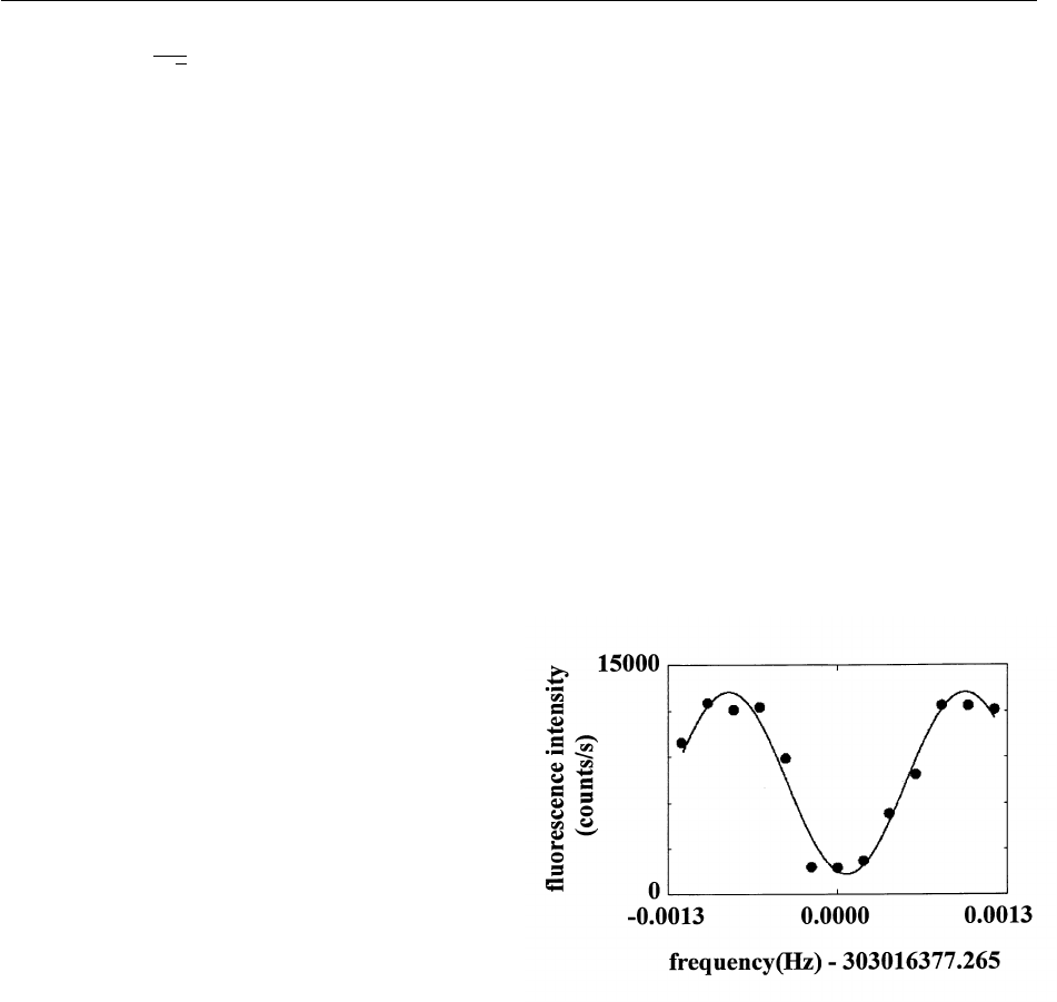
Volume 103, Number 3, May–June 1998

Journal of Research of the National Institute of Standards and Technology

final

Ï2

↓l

↓

(x)+↑l

↑

(x)

↓

(x)=[C

↓,0

) 2 e

)

↓,1

)]0l

2 isin

1,2

)

↓,2

)1l (82)

i=2

cos

i21,i

↓,i

)

2 isin

i,i+1

)

↓,i+1

)

il,

where

and

are the phases (Eq. (23)) of the analysis

pulses relative to the pulses used to create the state

(0). We now measure the probability P

↓

of finding the

atom in the ↓l state and obtain

↓

C

↓,0

)

+ C

↓,1

)

2 2Re[iC

↓,0

↓,1

i=2

C

↓,i

)

, (83)

where D

≡

. In this expression, we have as-

sumed all cross terms of the form C

↓,i

↓,i+1

for i $ 1

average to zero over many measurements; this will be

true if decoherence is caused by some process which is

uncorrelated with the creation and analysis pulses.

We fi n d kRe(C

↓,0

↓,1

)l =

/2kP

↓

(p) 2 P

↓

(0)l and

kIm(C

↓,0

↓,1

)l =

/2kP

↓

(p/2) 2 P

↓

(2p/2)l. Therefore,

from measurements of P

↓

for four values of D

,we

measure the coherence (C

↓,0

↓,1

) (or

0,1

), the off-di-

agonal matrix element of the motion after time t

). If

necessary, we can find the amplitudes C

↓,0

) and

C

↓,1

) by applying the blue sideband to

) for a

time

and reducing P

↓

(

) as described in Sec. 3.2.1.

4.2 Internal State Decoherence

For many years, one of the principal applications of

the stored-ion technique has been for high-resolution,

high-accuracy studies of internal state structure of

atomic ions. This capability can be applied for use in

atomic clocks (for reviews of efforts from a number of

laboratories, see Refs. [242] and [243]). High resolution

and accuracy are obtained because ions can typically be

stored for long times (many hours or days) with minimal

perturbations to their internal structure from electric

and magnetic fields.

Energy level shifts caused by electric fields (Stark

shifts) are usually small and, in many cases, magnetic

field level shifts can be controlled well enough; these

properties lead to very weak decoherence between inter-

nal state superpositions. As an example, in Fig. 7, we

show a spectrum taken of a particular hyperfine transi-

tion in

ions [76]. This resonance, obtained with the

Ramsey method of separated fields [173], has a

linewidth of less than 0.001 Hz (at a frequency

2p . 303 MHz) and corresponds to a coherence time

between the two internal levels of the transition of more

than 10 minutes. (We could independently establish that

the noise apparent in Fig. 7 was primarily caused by the

fluctuations in the oscillator driving the transitions and

not due to decoherence of the

internal levels.) More

recently, a slightly narrower resonance was reported by

Fisk et al. [244]. This resonance was observed on a

much higher frequency hyperfine transition in

171

(. 12.6 GHz) which resulted in a Q factor of 1.5 3 10

(Q ≡ transition frequency/linewidth). For levels sepa-

rated by optical energies, very long coherence times are

also possible because of the very long radiative lifetimes

of particular optical levels. So far however, observed

coherence times have been limited by the linewidth

of the probing lasers to a few tens of hertz

[235,245,246,247].

Fig. 7. Ramsey signal of the 2s

1/2

= 2

/2, M

/2) →

1/2

(2 3/2, +

/2) hyperfine transition in

at a magnetic field of

0.8194 T). This resonance was obtained using a free precession time

of 550 s. The data are the result of one sweep (one measurement per

frequency point). The fluctuations in the data were due to the instabil-

ity of the reference oscillator used to take the spectrum. These kinds

of measurements indicated that the coherence time for superpositions

between the two hyperfine states (which could be used as qubit levels)

was longer than 10 min [76].

These relatively small rates of decoherence indicate

that quantum states considered for clock transitions are

also attractive as qubit levels for a quantum computer.

However, the long coherence times obtained in the spec-

troscopy experiments were obtained under special con-

ditions which may not always be compatible with their

use in quantum logic. Therefore, in this section, we

consider various sources of internal state decoherence

and how they might be controlled.

290

Volume 103, Number 3, May–June 1998

Journal of Research of the National Institute of Standards and Technology

4.2.1 Radiative Decay

A fundamental limit to internal state coherence is

given by radiative decay. In general, we must consider

decay from both levels of a two-level system; for sim-

plicity, and as is often the case, we will assume the lower

state is stable.

For electric dipole radiation, the decay rate from up-

per state 2l to lower state 1l is given by

rad

k2

1l

/(3p

) where

≡ (E

2 E

and

denotes the atomic dipole operator. For magnetic dipole

radiation, we have

rad

k2

1l

/(3p

). For

hyperfine transitions, which decay by magnetic dipole

radiation, we make the approximation k2

1l .

the Bohr magneton. If we assume

/2p = 10 GHz, then

rad

. 10

212

, clearly small enough for the discussion

here. For optical electric dipole transitions, we make the

approximation k2

1l . qa

where 2 q is the elec-

tron charge and a

is the Bohr radius. If we assume

/2p =10

Hz (

= 300 nm), we find

rad

. 7.5 3 10

, which is much too fast for our purposes. However,

as is well known, a number of trapped-ion species have

first excited optical levels which are metastable. A well-

studied case is Ba

for which the first excited

5/2

state

radiatively decays by electric quadrupole radiation. It

has lifetime measured to be about 35 s [95,248,249,

250]. Other ions also have metastable optical levels

which are interesting for the purposes here. Some of

these are considered by Hughes et al. [63,64] and Steane

[60]. Lifetime measurements of various ions have been

compiled and reviewed by Church [251].

4.2.2 Magnetic Field Fluctuations

In the absence of purposely applied electromagnetic

fields which provide the logic operations, uncontrolled

fluctuating external magnetic fields are expected to give

the primary contribution to internal state decoherence.

Decoherence results from the fact that the energy sepa-

ration between two levels of interest depends on the

external magnetic field B. In most cases, it will be

possible to express the transition frequency between two

levels to sufficient accuracy by

+ d



B

(B 2 B

)



B

(B 2 B

)

, (84)

where B

is the average magnetic field and

is the

transition frequency for B = B

The effects of a fluctuating magnetic field depend on

the spectrum of the fluctuations. We first assume the

typical case that the fluctuations are slow enough to be

considered quasi-static during the time of a single oper-

ation

. A common source of low frequency fluctua-

tions which would typically fit into this category are

sinusoidal field fluctuations due to unbalanced currents

in ac power lines. Therefore, in the spin-

/2 analog, we

assume

internal

[1 +

(t)], (85)

where

<< (

)

. For this Hamiltonian,

Schro¨dinger’s equation yields

↓

(t 2 t

)=C

↓

(t)

↑

(t 2 t

)=C

↑

(t)

, (86)

(t) ≡

t +

(t')dt'

In a sequence of logic operations,

(t) must be small

enough or be taken into account (see also Sec. 4.3.2).

As a second case, we assume the magnetic field varies

rapidly; specifically, we assume B varies sinusoidally:

B 2 B

= DBcos

t where

>> 1/

.Wefind



B

DBcos



B

(DB)

(1 + cos2

t). (87)

The term [

/B

]DB

/4 on the right side of this ex-

pression is a frequency shift which can be absorbed into

the definition of

if DB remains constant. For simplic-

ity, assume that one of the cosine terms in Eq. (87)

dominates so that d

sinusoidally oscillates at

or 2

so that

(t)=

cos

t in Eq. (85). The effects

of this fast modulation can be seen if we consider apply-

ing external radiation near the carrier frequency

the internal state transition. Schro¨dinger’s equation

leads to expressions similar to those of Eqs. (17) which

take the form (for

=0)

↑,n

= 2 ie

sin

n,n

↓,n

= 2 ie

2i(

sin

n,n

↑,n

, (88)

where

≡

.Wehave

6ih

sin

= J

(

)

(

)cos2

t + J

(

)cos4

t + ...

6 2i

(

)sin

t + ...

. (89)

291

Volume 103, Number 3, May–June 1998

Journal of Research of the National Institute of Standards and Technology

where J

(X)istheith Bessel function with argument X.

For

>> 1/

n,n

, the sinusoidally varying terms

on the right average to zero (as in the rotating wave

approximation). Therefore the wavefunction evolves just

as in Eq. (25) except we must replace 

n,n

 by



n,n

J

(

). Since the J

factor can be absorbed into

the definition of

, this steady modulation should not

cause a problem. An important source of high-fre-

quency magnetic fields is from the currents in the elec-

trodes which oscillate at the trap drive frequency

The gate demonstrated in Ref. [17] had a strong sen-

sitivity to magnetic field fluctuations since the qubit

frequency and the auxiliary transition frequency had a

dependence 

/B .

. 10

Hz/T. If this scheme

is used in future experiments, sufficient magnetic

shielding must be provided. Alternatively, the magnetic

field dependence can be minimized by operating at a

magnetic field where the transition frequency becomes

independent of magnetic field to first order (making the



/B terms in Eq. (84) and (87) vanish). For example,

most atomic clocks are based on hyperfine transitions in

ground electronic

1/2

states, where the nuclear spin I is

half integral (

/2, 3/2, 5/2, ...). In these cases, where the

total angular momentum (F = I + S) is integer, the

(F,m

=0)↔ (F',m

= 0) transition is first-order field

independent for B . 0. These particular transitions

may not be useful in the applications discussed here

since other transition frequencies (for example,

(F,m

=0)↔ (F',m

= 6 1) transitions) will be very

close to that of the (F,m

=0)↔ (F',m

= 0) transition

frequency as B→0. This may cause unwanted cou-

plings to these other levels. At optical frequencies, sim-

ilar first-order field independent transitions in ions have

been used in frequency standards [235]. However, other

hyperfine and optical transitions become first-order

field independent at nonzero magnetic field, and their

frequencies are separated from competing transitions

(see, for example, Refs. [76] and [189]).

For quantum logic, storing qubit information in two

states whose energy separation is first-order field inde-

pendent therefore appears to be attractive. However, the

conditional dynamics which is central to quantum logic

may necessitate a transition to an auxiliary state. In the

notation of Sec. 3.3, a transition between the ↑l and

auxl levels will have a transition frequency which will,

in general, not be first-order field independent if the

↓l →↑l transition frequency is field-independent.

Therefore, if the external field fluctuates, the fidelity of

this operation will be compromised. As an example,

suppose quantum logic is performed on a collection of

ions using the 2s

1/2

m

= 2 3/2,m

=1/

2l ≡ “↓l”and2 1/2,1/2l ≡ “↑l” levels as qubits

(strong-field state representation). With these designa-

tions, level ↓l has a higher energy than level ↑l. These

are the same levels as those used for the clock reported

in Refs. [75] and [76]; the transition frequency

2p . 303 MHz is first-order field independent at a field

of B

. 0.8194 T. At this magnetic field, the transition

frequency has a second-order dependence of d

2p . 2 5.2(dB/B

)

MHz. Therefore, a field fluctua-

tion of dB =10

T from B

leads to a frequency offset

of the transition of only about 80 mHz. For the first CN

gate described in Sec. 3.3, we could use 2p transitions

between the ↑l and “auxl” ≡1/2,1/2l level. How-

ever, this transition has a first-order dependence on

magnetic field at 0.8194 T given by (

/2p)/

B . 2 22 MHz/T. Therefore if the field shifts by

dB =10

T, this will cause a shift of this transition

frequency of

/2p = 2 2200 Hz. Similar consider-

ations must be applied to quantum logic using other ions

such as

201

ions where the splittings between hyper-

fine transitions are much higher [252]. Since it will be

difficult to find two field-independent transitions at the

same field, it may be advantageous to use logic gates

which require only one internal state transition as in the

second and third gates described in Sec. 3.3.

4.2.3 Electric Field Fluctuations

In Sec. 4.4, we treat the effects of electric fields from

the applied laser beams; in this section we treat the

effects of other electric fields. Electric field shifts are

likely to be less important as a source of internal state

decoherence than shifts due to external magnetic fields.

First, electric-field shifts are second-order in the field,

except for exceptional cases involving nearly-degenerate

states of opposite parity. Second, the fields are relatively

small at the site of the ion. In analogy to Eq. (84), we

have

+ d



E

E=0

, (90)

where E is the magnitude of the electric field. Unlike

Eq. (84), the expansion is made around E = 0, rather

than a nonzero value E

, since, as noted previously, the

mean value of E is zero for an ion in a trap. If it were not

zero, then the ion would have a mean acceleration and

would not be spatially localized. Of course, the ion must

experience an average electric field to counteract the

force of gravity, but this field is extremely small. For an

ideal rf trap, such as one in which the rf potential is

described by Eq. (1), and in which there are no stray

static electric fields, the ions are attracted to the line

along which the rf electric field is zero. In this case, the

mean-squared electric fields due to confinement experi-

enced by cooled ions are very small. If stray fields are

present, the mean-squared electric field seen by the ions

292

Volume 103, Number 3, May–June 1998

Journal of Research of the National Institute of Standards and Technology

will be nonzero and can be significantly larger [228].

The stray fields can be reduced by applying potentials to

compensation electrodes; to some extent this is neces-

sary anyway for the efficient laser cooling. It should be

possible to reduce the rms electric fields from the elec-

trodes and neighboring ions to less than 1 V/cm. We

note that rms electric fields of about 8 V/cm are present

at room temperature, due to the blackbody (thermal)

electromagnetic field. Since the spectrum of this field is

dominated by infrared frequencies and because it is

steady, this should lead only to a small ac Stark shift

[253].

We briefly consider two cases that have been dis-

cussed for ion trap quantum computation: narrow opti-

cal transitions between the ground and a metastable state

and transitions between ground-state hyperfine sublev-

els. For an optical transition between two energy levels,

the energy shift, derived from perturbation theory, is

roughly (qa

)

/DE, where qa

is the product of the

proton charge and the Bohr radius, that is, a typical

electric-dipole matrix element, DE is a typical energy

difference between one of the two levels and another

which is connected by the electric-dipole operator, and

E is the electric field. For the case of the Ba

1/2

-to-

5/2

transition which has a wavelength of 1.76 mm,

this expression predicts a shift d

/2p of approximately

3 mHz for E = 1 V/cm, if DE is taken to be the 6s

1/2

-to-6p

1/2

energy difference. This is in rough

agreement with the experiment of Yu et al. [254]. Simi-

lar values of d

are estimated for the 5d

1/2

→

5/2

transition in

199

[228]. Transition fre-

quencies between hyperfine levels, such as those used in

the NIST single

ion experiments, are even less

sensitive to electric fields, since, to a good approxima-

tion, an electric field shifts all sublevels of the hyperfine

multiplet by the same amount. A differential shift be-

tween the sublevels arises in third-order perturbation

theory [253]. For

, for example, the fractional shift

between hyperfine sublevels is approximately

2 4 3 10

218

for E = 1 V/cm [255].

So far, we have considered only electric dipole shifts,

that is, the shifts that are due to a uniform electric field.

An electric quadrupole shift, which is proportional to

the product of the electric quadrupole moment of the

state and the applied electric field gradient, may also be

present. The shift d

is given approximately by

E

r

, (91)

where Q

is the atomic quadrupole moment and E

/r

is a typical component of the electric field gradient

tensor, such as E

/z. The precise value depends on the

whole electric field gradient tensor and the details of the

atomic state. There is no quadrupole shift for S-states or

for other states with electronic angular momentum

J < 1, like the

states in the Group IIIA ions, such as

[256]. The trap rf electric fields have gradients, but,

since they oscillate sinusoidally, they average to zero.

Static electric field gradients due, for example, to patch

effects, or the static potential to confine ions along the

axis of a linear trap [Eq. (2)] would be more of a prob-

lem. For a typical value of Q

=10a

, and an electric

field gradient of 10 V/cm

, d

/2p ≈ 0.7 Hz. Fluctua-

tions in this (small) shift will probably be small com-

pared to those of magnetic field shifts. Electric field

gradients due to neighboring trapped ions will also be

present [257]. Consider an ion at position x = y = z =0.

The electric field gradient component E

/z due to ions

having charge q, located at x = y =0,z = 6 d is 2 q/

). For d =10mm, this is 575 V/cm

. However, this

should be relatively constant, since the spacing between

ions is determined by the trap fields, which must be kept

nearly constant if motional decoherence is to be avoided.

Thus, they may lead to energy shifts, but not to decoher-

ence.

Garg [58,59] has considered the decoherence of inter-

nal states of ions due to fluctuating electric fields in-

duced by the reservoir of vibrational modes of a string

of trapped ions. Such decoherence is present even if the

modes are in the ground state, because of zero-point

motion. This form of intrinsic decoherence was found to

be negligible, at least for the specific case in which the

1/2

and the 5d

5/2

states of Ba

are used to store the

qubits. For a string of 1000 ions, the decoherence time

was found to be around 10

2 10

times longer than the

natural lifetime of the upper state, which is 35 s.

4.3 Logic Operation Fidelity and Rotation Angle

Errors

The third and perhaps most important class of deco-

herence involves imperfections in the logic operations.

Ideally, a quantum computation transforms an initial-

ized state vector

(0) to U

ideal

(0), where

ideal

= exp[2 iH

ideal

] (with H

ideal

time independent)

is the unitary evolution operator without errors. In prin-

ciple, both U

ideal

and the corresponding interaction

Hamiltonian H

ideal

operate on the Hilbert space formed

by the ↓l and ↑l states of the L qubits. In practice, for

the case of trapped ions, the physical implementation of

logic gates requires that we must include at least the 0l

and 1l states of the chosen motional mode and perhaps

an internal auxiliary state (Sec. 3.3). If decoherence

mechanisms cause other states to be populated, the

Hilbert space must be expanded. Although more

streamlined algorithms may be available, the operator

ideal

can always be broken up into fundamental single

and two-bit quantum gates [140,155,156,157]; for sim-

plicity, this will be assumed in what follows.

293

Volume 103, Number 3, May–June 1998

Journal of Research of the National Institute of Standards and Technology

In the previous sections, we have concentrated on the

decoherence of the state vector

due to environmental

coupling, in the absence of purposely applied additional

fields. Here, we treat decoherence due to imperfections

in the evolution operator U

ideal

which is implemented by

these additional applied fields. We break this decoher-

ence into two categories: (i) errors or noise in the (clas-

sical) gate parameters (that is, the rotation angles

and

n',n

t in Eq. (23)) which result in undesired evolution

and, (ii) coupling to the environment induced by the

gates (for example, spontaneous emission induced by the

applied fields). In some cases, we can model noisy logic

gates by considering an ensemble of gates whose

parameters are statistically distributed. This allows a

simple characterization of several candidate noise

sources.

The final step in an ideal quantum computation is a

probabilistic measurement of all the quantum bits,

which yields a given L-bit number k, or equivalently, the

state k, with probability P

= kkU

ideal

(0)l

(k = 0,1,2,...,2

2 1). A particular quantum computation

is thus completely characterized by the vector of proba-

bility amplitudes A

= kkU

ideal

(0)l. The usefulness of

a quantum computer algorithm relies on the coherent

interference of the probability amplitudes, resulting in

only a small fraction of the 2

possible numbers with

appreciable measurement probability. If the actual evo-

lution operator U contains imperfections, the probabil-

ity amplitude vector is instead B

= kkU

(0)l Þ A

We characterize the fidelity of a computation by the

expression

F =

kU

ideal

(0)U

(0)l



k=0



, (92)

where the average is performed over any random vari-

ables affecting the operator U. Roughly speaking, F is

the probability that errors in the operator U do not affect

the result of a computation, with F = 1 representing

error-free computation. This characterization of the fi-

delity follows the approach of quantum trajectories

[258,259]. A quantum computation can be interpreted as

the evolution of a complicated path through Hilbert

space. If the operations comprising the computation are

imperfect, the path of computation bifurcates into a

superpositions of the correct path and incorrect path

[260]. In this model, the fidelity F is just the probability

that the correct path has been followed. Schemes for

complete characterization of a quantum process in terms

of a input-output matrix have been proposed in Refs.

[261] and [262]. This approach would be able to charac-

terize the fidelity of any of the operations discussed

here. It can also be used to test for decoherence of the

internal and motional states, by use of time delays be-

tween state preparation and application of the diagnos-

tic.

An adequate characterization of the effects of noise in

a quantum computation requires knowing the type of

noise processes present, and application of this noise to

a specific computational algorithm on a specific input

state. This is most straightforwardly accomplished using

numerical simulations [1,263–266]. Here, we do not

treat any specific algorithms, but will attempt to make

some general observations on particular sources of logic

operation errors and how these errors accumulate after

many operations.

4.3.1 Accumulated Errors

Each successive operation in a quantum computation

based on the Cirac/Zoller trapped-ion scheme can be

regarded as a rotation between two states Al

nl and

A'l

n'l in a multidimensional Hilbert space where

Al

and A'l

are from ↓l

, ↑l

,orauxl

and nl and

n'l are from 0l or 1l of the selected motional mode.

Before the kth operation, assumed to be applied to the

jth ion, we can, to a good approximation, write the

wavefunction as

k21



k21,



k21,

l +

k21



k21,



k21,

k21



k21,



k21,

l, (93)

where 

k21,

and 

k21,

are the basis states for the

rotation (for example, the ↑l

1l and auxl

0l states

required to carry out step 1b of Sec. 3.3). The state



k21,

is the part of the wavefunction for the jth ion

which does not include states involved in the rotation

(for example, the ↓l

state). The states 

k21,



k21,

l,and

k21,

l are states which include other ions

and, because of gate imperfections, may involve states

outside the Hilbert space spanned by the ↓l, ↑l,

and auxl internal states, and 0l and 1l motional

states. We choose k

k21,



k21,

l = k

k21,



k21,

l =

k21,



k21,

l = 1 so that 

k21



+ 

k21



+ 

k21



1. From Eq. (23), the “actual” kth operation can be

written as

(

cos(

) 2ie

sin(

)

k21

2ie

sin(

) cos(

)

k21

(94)

where, to simplify notation, we have chosen

n',n

and

<< p are the errors in the ampli-

tude and phase of the rotation. We can write

294

Volume 103, Number 3, May–June 1998

Journal of Research of the National Institute of Standards and Technology

= R

+ DR

, (95)

where R

= R

cos

≡ R

(

, 0)] is the ideal kth op-

erator and

has terms which are first order (and real) in

and

. Nevertheless, we might expect that the overall fi-

delity has errors which depend only quadratically on

and

since a general computation may approximate a

sequence of nearly random rotations on a multidimen-

sional Hilbert space. To see how this might come about

we express a general computation consisting of M oper-

ations as

O = R

(M21)a

...R

. O

+ O

, (97)

where

≡ R

M21

...R

≡ [R

...R

]+[R

...DR

]...

+ ...[R

M21

...R

]+[DR

M21

...R

], (98)

≡ R

...R

+ R

...DR

...

+ ...DR

M21

M22

...R

+ DR

M21

M22

...R

and where we have neglected terms which are higher

than second order in

and

. In this notation, the ideal

computation is given by the operator

ideal

= R

...R

. (99)

For the fidelity, we need to calculate

(0)O

†

ideal

O 

(0)l = k

(0)O

†

ideal

+ O

)

(0)l where we will neglect terms of third order

and higher in {DR

}. For the first term, we find

(0)O

†

ideal



(0)l.1 2

i=1

. (100)

For the second term, we have a sum of M terms; the kth

of which is given by

(0)O

†

ideal

M21

...DR

...R



(0)l

(0)R

†

...R

†

k21

...R



(0)l (101)

= k

k21,0

R

†



k21,0

❘

where

k21,0

corresponds to the wavefunction repre-

sented in Eq. (93) for the ideal case. We find

k21,0

R

†



k21,0

l.2

sin

[

k21



+ 

k21



]

2 i[(

k21



2 

k21



)(

cos

+ sin

)

sin

(102)

+2Re[

k21

](

sin

cos

)

2 2Im[

k21

](sin

cos

)

cos

The third term k

(0)O

†

ideal



(0)l is straightfor-

ward to evaluate and is clearly second order in

and

. Even though the imaginary term in Eq. (102) has

terms linear in

and

, when the fidelity F is calcu-

lated, these terms add only in quadrature so the kth

operation gives only a contribution of second order in

and

. Therefore, in general, we have

F . 1 2

k=0

+ C

, (103)

where the coefficients C

, C

1. For general

computations involving many operations M in a large

Hilbert space, it might be expected that the errors in

rotations are distributed in an approximately random

fashion. In this case, we would expect the fidelity to be

approximately given by F . 1 2 M(F

+ F

) where

and

are characteristic of the errors for

all operations and F

, F

1. In the case ampli-

tude errors (

) dominate, then the maximum number of

operations before the fidelity drops appreciably below 1

is M

max

. 1/

. For example, laser intensity fluctuations

on the order of 1 part in 10

would give M

max

. 10

.At

the other extreme, the errors might add coherently in

some cases. These operations could conspire to give

contributions to the fidelity that goes as (

)

.We

can illustrate this with a simple example. Assume that

an intended rotation

has an error

<< p. The state of

the system before application of this rotation can be

expressed by Eq. (93). From Eq. (92) we find F =

cos

(

/2)(

k21



+

k21



)+4[Re{

k21

exp(i

)}]

sin

(

/2). The existence of the second term only serves

sin

2 1)sin

cos

sin

≡ 2

. (96)

2 1)sin

cos

sin

295

Volume 103, Number 3, May–June 1998

Journal of Research of the National Institute of Standards and Technology

to improve the fidelity, so at worst (when

=1 or

= 1), the fidelity of this single operation is given by

cos

(

/2) . 1 2 (

)

/8. Now suppose that a second ro-

tation

about the same axis has error

. A similar

analysis shows that when these two operations are ap-

plied in succession, a worst case for the fidelity is given

by F = cos(

/2 +

/2) . 1 2 (

)

/8. Similarly,

for rotations on M bits, the worst case fidelity is given

by F = cos(

/2) so that the errors could accumulate

linearly. Most likely, this case will correspond to rather

uninteresting computations and one can generally expect

that the errors will accumulate in a way which is be-

tween random walk and linear.

The effects of operation errors (

) have been

observed in simulations of quantum computations to

factorize small numbers [263,266]. If the errors fluctu-

ate randomly about the correct value, the fidelity is

given by a simple expression which is essentially the

same as Eq. (103) for F . 1 [266]. However, for con-

stant errors the fidelity indicated by the simulations is

somewhat worse indicating that the computational al-

gorithms cannot be assumed to be rotations about axes

chosen pseudo randomly. Therefore, the simulations in-

dicate that requirements on systematic offsets are more

stringent than the requirements on random fluctuations

from operation to operation.

4.3.2 Pulse Area and Phase Fluctuations

As in the last section, we will consider two sources of

noise: (1) those which result in offsets from, and fluctu-

ations in, the ideal Rabi frequencies [for example, off-

sets and fluctuations of

n',n

t in Eq. (21)] and (2) those

caused by phase fluctuations between applications of

separate operations to a particular ion [fluctuations from

some constant value of

in Eq. (21)].

We first make some remarks regarding the coherent

evolution between two states of the system which com-

prise the basis states for a single operation. First, there

are a number of methods of coherently transferring pop-

ulation between a two level system with radiation, in-

cluding constant amplitude Rabi pulses as represented

by Eqs. (21) and (23), adiabatic rapid passage [267], and

adiabatic transfer via dark states [268–270]. The advan-

tage of the last two techniques is that for p pulses, their

efficiency does not depend critically upon the pulse area

(Eq. (104) below) of the applied field. However, for

rotations other than p, this advantage is lost. Moreover,

for these techniques to work with high efficiency, par-

ticularly simple atomic level structures are required and

coupling to any off-resonant levels can potentially con-

taminate the transfer. For example, adiabatic transfer

can be extremely efficient between ground state hyper-

fine levels if the transfer occurs only through a single

excited (electronic) state. However, in practice, other

excited states are driven by the coupling (laser fields)

thereby affecting the fidelity of the transfer [271]. Fur-

thermore, the high powers required for adiabatic rapid

passage and adiabatic transfer aggravate decoherence

from spontaneous Raman scattering (Sec. 4.4.6.4).

Therefore, we will only consider the case of Rabi

pulses, where population is transferred by applying a

resonant field with a well-controlled amplitude envelope

and duration.

When a resonant radiation field is applied to a two-

level system, the resultant unitary transformation is

given by Eq. (23). We can further generalize this expres-

sion replacing

n',n

t by

n',n

(t)/2 where

n',n

(t)=2

t'=0

n',n

(t')dt' (“pulse area”). (104)

The factor of two in this equation is introduced so that

the condition e

n',n

(t')dt' = p/2 corresponds to a p pulse

of the effective Bloch vector. Here, as opposed to the

situation assumed in Sec. 2.3.1 (where the coupling

radiation was assumed to be turned on instantaneously,

left at constant amplitude, and then turned off instanta-

neously), we now allow the coupling radiation to be

turned on and off gradually. This more closely approxi-

mates a real experimental situation and can be advanta-

geous since the spectrum of

n',n

(t) can be tailored to

suppress off-resonant transitions (Sec. 4.4.6). Here, we

call

n',n

the pulse area of the applied radiation and

n',n

(t) the Rabi frequency envelope. If the applied

pulse area is noisy or set incorrectly, then the output

state will fluctuate from it’s ideal value as discussed in

the previous section.

We must also consider detunings between the applied

frequencies and resonant frequencies of the ions [in Eq.

(21)] and phase fluctuations between successive opera-

tions on the same ion [fluctuations in

in Eq. (21) from

operation to operation]. This could occur from fre-

quency or phase fluctuations in the applied fields or

fluctuations in the ion internal or motional frequencies.

For frequency fluctuations, we consider that for a given

operation on ion j,

(t) is slowly varying over the time

of a single operation (Sec. 4.2.2). In the limit that detun-

ings are small, the dominant effect can be characterized

by assuming that

= 0 for each operation, but that

different phases

(t')dt', (105)

are present for successive applications of the same oper-

ation. In this expression, t

is the time that the first

operation is applied at ion j and t

is the time of the kth

operation (applied to the jth ion).

296

Volume 103, Number 3, May–June 1998

Journal of Research of the National Institute of Standards and Technology

4.4 Sources of Induced Decoherence

Below, we consider various sources of fluctuations

and decoherence caused by the logic operations and how

these might be evaluated and controlled in experiments.

First, we are interested in controlling the accuracy and

stability of the Rabi pulse are

n',n

given by Eq. (104)

and the accumulated phase as expressed in Eq. (105).

Since gates will most likely be implemented with laser

transitions we will examine laser intensity and timing

fluctuations.

4.4.1 Applied Field Amplitude and Timing

Fluctuations

Fluctuations in the laser intensity at the site of a given

ion can arise from both fluctuations in the relative posi-

tion of the beam with respect to the ion and fluctuations

in laser power. Laser/ion position stability is particularly

important since the Cirac/Zoller scheme of quantum

logic assumes that ions in an array be selectively ad-

dressed, thereby requiring a high degree of control of

the laser beam spatial profile (Sec. 4.4.4). Of course, the

simplest method for minimizing position fluctuations is

to employ mechanically stiff mounts for the optics and

ion trap electrodes, and have the laser source as close as

possible to the ions. A quadrant detector indexed to the

trap electrodes and placed near the ion may also be used

to actively stabilize the beam position by feeding back to

a galvanometer or acousto-optic modulator. If optical

fibers are used to deliver laser beams to the ions, posi-

tion fluctuations between the fiber and the ions could be

made small; however, we must also consider position

fluctuations between the laser source and the input to

the fiber. If the position tolerances can be adequately

controlled, the dominant source of intensity noise at the

ion would likely be given by fluctuations in optical

power and laser mode. Here, we estimate limits on laser

amplitude noise.

If we assume the laser fields responsible for quantum

logic operations are coherent states, the fundamental

noise floor is photon shot noise. For a laser beam of

average power P

, the fractional level of shot noise is

= Î

, (106)

where

is the (optical) photon frequency,

is the time

the radiation is applied, and, for simplicity, we assume

square pulse envelopes as in Eq. (23). Of course, lasers

seldom produce amplitude noise at the photon shot-

noise limit. Almost all laser sources have significant

amplitude noise in the 10 Hz to 10 kHz range due to

acoustic vibrations which, for example, affect the laser

cavity resonators. Much of this noise can be removed by

active power stabilization, where a beamsplitter directs

a portion of the laser power to a photodetector, and an

error signal is derived and fed back to an upstream

modulator or, in the case of a diode laser, directly to the

amplitude of the laser source [272,273]. The limiting

noise of this stabilization scheme is degraded slightly by

the imperfect quantum efficiency of the photodetector

as well as the beamsplitter. If the beamsplitter directs a

fraction

of the input optical power to the stabilizer

(which then gives an optical power P

. (1 2

di-

rected to the ion), and the quantum efficiency of the

photo detector is

det

, the limit of fractional power noise

in the logic pulse is (assuming no added electronic noise

in the feedback loop)

$ Î

det

(1 2

)

. (107)

For a laser wavelength of 313 nm, and assuming

= 0.5

and

det

= 0.5, we have dP

$ 2.3 3 10

)

21/2

For1Wofusable laser power and

=1 ms, this

corresponds to a fractional power fluctuation of

$ 2.3 3 10

This estimate applies only to the laser power fluctua-

tions at the beamsplitter and assumes no additional noise

is introduced between the beamsplitter and the photo

detector or the beam splitter and the ions. Typically, the

usable part of the laser beam must be directed further

through optics, the air, and a window to the vacuum

envelope enclosing the ion trap. Fluctuating etalon ef-

fects in the optics and air currents may therefore seri-

ously increase the power fluctuations beyond Eq. (107).

The effects of (Gaussian) noise on laser intensity have

been treated by Schneider and Milburn [274]. These

effects show up in a well-characterized way for transi-

tions involving Fock states.

Fluctuations in timing errors may also be important.

Clearly, fractional fluctuations in the duration of laser

pulses will correspond directly to the same fractional

fluctuations in the desired value of

n',n

. If we require

fractional fluctuations of 10

n',n

, then we require

timing precision of 1 ps on a 1 ms pulse. Similar consid-

erations apply to the stability of pulse envelope shapes.

For both amplitude and timing fluctuations, it may be

possible to sample a portion of the beam used for logic

and apply it to a “check bit” ion. The response of this ion

could then be used to monitor and control the amplitude

and timing of the pulses.

4.4.2 Characterization of Amplitude and Timing

Fluctuations

In practice, it may be easiest to characterize the am-

plitude and timing fluctuations with a power detector

297

Volume 103, Number 3, May–June 1998

Journal of Research of the National Institute of Standards and Technology

placed as close as possible to the position of the ions.

However, it would be useful to characterize these effects

using the ions themselves. One possibility is to observe

the sinusoidal Rabi oscillations predicted by Eq. (21).

For example, for a single ion initially prepared in the ↓l

state, we can record the probability P

↓

(

) of detecting

the ion in the ↓l state after the laser is applied to the ion

for time

. From Eq. (23), if we first prepare the ion in

the ↓,nl state and if the power is constant,

↓

(

)=C

↓,n



= cos



n',n

t =

/2[1 + cos2

n',n

t]. In

Fig. 2, we show this type of curve for n = 0 and n' =1.

This plot includes a decay due to decoherence. Here, we

consider decoherence caused by specific types of noise.

We will cast the results in terms of fluctuations in

n',n

however, they may easily be converted to corresponding

time fluctuations since we are really interested in fluctu-

ations in the net rotation angle given by Eq. (104). For

simplicity of notation, in this section, we write

n',n

First assume that

fluctuates slowly so that it is

constant over the time

for an individual measurement

of P

↓

(

) but fluctuates over the time taken to make an

average measurement of kP

↓

(

)l. We characterize power

fluctuations by a spectrum D(

)of

values

around the desired value

.Wehave

↓

(

)l =

[1 + cos2

]D(

)d(

(108)

We illustrate with two possibilities for D, finding

↓

(

)l =

1 + cos2

22(D

rms

)

for

Ï2pD

rms

(109)

↓

(

)l =

1 + cos2

1+2(D

rms

)

for

rms

Ï2



rms

❘

where (D

rms

)

≡ k(

)

l. In both cases the contrast

of the signal drops about a factor of two for

. 1/

rms

. Although the second choice of D(

)

seems less physical, it indicates the exact spectrum of

the noise may not be important for a qualitative test. If

we need to detect fluctuations of order D

rms

, then

we must measure P

↓

after approximately

/2p .

/(2pD

rms

) Rabi cycles. For example, if we require

sensitivity D

rms

. 10

, we need to make measure-

ments of P

↓

(

) after about 1500 Rabi cycles.

If, instead, the intensity fluctuates slowly compared

, but fast compared to the time

, kP

↓

(

)l isaless

sensitive test of the fluctuations since their effects tend

to average out. In order to show the effects of high-fre-

quency fluctuations of

for a simple case, we consider

a sinusoidal time variation:

(t)=

+ D

sin(

amp

t +

), (110)

amp

is the modulation frequency of the Rabi amplitude

(t). This analysis should, at least, yield the dependence

on the amplitude and frequency of the fluctuations. The

measured quantity P

↓

(

)isgivenby

↓

(

[1 + cos

(

)], (111)

where the rotation angle

(

) is given by Eq. (104)

which, here, takes the form

(

)

(t)dt =

+ D

sin(

amp

t +

)dt

(112)

amp

[cos

(1 2 cos

amp

) + sin

sin

amp

This yields

↓

(

1 + cos

amp

[cos

(1 2 cos

amp

) + sin

sin

amp

]

1 + cos(2

)cos

amp

[cos

(1 2 cos

amp

) + sin

sin

amp

]

(113)

2 sin(2

)sin

amp

[cos

(1 2 cos

amp

) + sin

sin

amp

]

298

Volume 103, Number 3, May–June 1998

Journal of Research of the National Institute of Standards and Technology

Since P

↓

(

) is obtained by repeating the measurements,

and since the phase

will be random from one measure-

ment to the next, we average over

If we assume that D

amp

 << 1, which is valid for a

small, high-frequency, modulation, then the integrands

can be expanded to second order in (D

amp

Aside from the fast oscillations due to the cos

amp

term, which might be difficult to observe, the effect of

the high-frequency fluctuations of

is to reduce the

visibility of the signal by 2(D

amp

)

. This result can

be averaged over a distribution D

(

amp

4.4.3 Applied Field Frequency and Phase

Fluctuations

A simple source of fluctuations is due to frequency or

phase fluctuations in the radiation that is used to carry

out the basic operations. Schneider and Milburn [274]

have considered a specific model of phase fluctuations

for ion experiments and calculate the corresponding

decoherence for operations of the type used in quantum

logic. If qubit energy levels are separated by optical

energies, the lasers that drive qubit transactions must

have the required frequency and phase stability. Given

the performance of current stable lasers [235,245,246,

247], this may be a problem for long computations. As

discussed in Sec. 2.3.3, optical stimulated-Raman trans-

actions provide the required strong field gradients

whereas the overall frequency sensitivity in the transi-

tions is dominated by the difference frequency of the

lasers, not the frequency of each laser. Since the two

Raman beams can be derived from one laser beam with

the use of frequency modulators, the frequency fluctua-

tions are dominated by those of the oscillator which

drives the modulator. The phase stability of these

sources can be high and does not appear to pose prob-

lems. For example, the data shown in Fig. 7 can be

↓

(

cos(2

)

cos

amp

[cos

(1 2 cos

amp

) + sin

sin

amp

]

(114)

sin(2

)

sin

amp

[cos

(1 2 cos

amp

) + sin

sin

amp

]

↓

(

≈

cos(2

)

1 2

amp

[cos

(1 2 cos

amp

) + sin

sin

amp

]

sin(2

)

amp

[cos

(1 2 cos

amp

) + sin

sin

amp

]

(115)

cos(2

)

1 2 2

amp

(1 2 cos

amp

)

❘

regarded as one test of the phase sensitivity of the

oscillator used to drive the indicated internal state tran-

sition. Stimulated-Raman transitions have the disadvan-

tage that they give rise to ac Stark frequency shifts as

indicated by the g

1,2



terms on the right side of

Eqs. (40). If these shifts are equal for both qubit levels,

the net shift is zero. If they are different, the effective

qubit frequency is shifted during the operation. This

must be measured and accounted for. The shift can be

tuned to zero by appropriately adjusting

and the

relative intensities and polarizations of the Raman

beams. A problem still exists if the Stark shifts fluctu-

ate; we examine the consequences of those fluctuations

here.

From Eqs. (40), the ac Stark frequency shift of the

qubit transition due to stimulated-Raman transition is

= 2 (g



2 g



, (116)

so that the shifted qubit frequency is given by

. We first consider the effects of frequency

fluctuations of the Raman beams. If the two beams are

derived from the same beam with the use of a modula-

tor, the frequency shift of the two laser beams will be

the same. Therefore, to a good approximation, we find

. 2 (d

)

where d

represents the fre-

quency shift of both laser beams. Typically,

>10

GHz, and frequency fluctuations of lasers can be con-

trolled to less than 1 kHz, so this source of error should

be small. Moreover, it is essentially absent if we tune

to be zero.

299

Volume 103, Number 3, May–June 1998

Journal of Research of the National Institute of Standards and Technology

More serious are fluctuations in laser intensity. We

will characterize these fluctuations by the correspond-

ing fluctuations in g

(~ square root of laser intensity).

From Eq. (116), we have

2 2

. (117)

As a worst case, we will assume fluctuations in g

and

are random and uncorrelated and, for simplicity, we

assume k(dg

)

l.k(dg

)

l ≡

, where kl denotes

an average over the spectrum of the fluctuations. There-

fore

k(d

)

l =4

(

). (118)

As discussed in Sec. 4.3.2, we assume the fluctuations

are slow compared to

, where

is the time of the

operation. In a particular operation, a frequency offset

gives rise to a phase fluctuation d

= d

.Itis

useful to characterize the effects of these phase fluctua-

tions by comparing their size relative to fluctuations in

rotation angles caused by the corresponding fluctuations

in the Rabi rates

n',n

. With the same assumptions re-

garding dg

and dg

,wehavek(d

n',n

)

l =2

Therefore, fluctuations in the overall rotation angle

n',n

[Eq. (104)] are given by k(d

n',n

)

l =2

. From these expressions we find

k(d

)

k(d

n',n

)

(

)

n',n

. (119)

For quantum logic, a worst case appears to be for side-

band excitation n' = n 6 1. If we assume the Lamb-

Dicke limit, we find

k(d

)

k(d

n',n

)

+ g

)

. (120)

From this expression, it is desirable to have g

. g

minimize the effects of d

relative to d

n',n

.Evenin

this case, rms phase fluctuations caused by Stark shifts

are worse than those caused by Rabi frequency fluctua-

tions by a factor of . 1/

. Most likely, however, fluctu-

ations in intensity will be dominated by fluctuations

from the primary laser from which both beams are

generated. Therefore we expect fluctuations to be corre-

lated dg

= dg

. When, in addition,

, the

phase fluctuations caused by Stark shifts will be less

than those caused by Rabi frequency fluctuations. If

these conditions hold true, it appears that stimulated

Raman transitions between two qubit levels separated

by fairly low (for example, hyperfine) frequencies are

superior to single-photon transitions between qubit lev-

els separated by optical frequencies. This situation

might change as laser oscillators become more stable.

In the above discussion, we have neglected the alter-

ation of the ion motional frequencies caused by the

superimposed dipole force potentials of the focussed

laser beams. However, if we assume the Raman beams

have waists w

which are approximately equal and that

the magnitudes of the projections of their k vectors

along the z axis are the same, it is straightforward to

show that the relative shift of (single trapped ion) secu-

lar frequencies for states ↓l and ↑l is approximately

equal to d

)

. Therefore, since z

<< w

, the fre-

quency shifting effects will be dominated by the shifts

of the internal states.

Phase fluctuations of the laser beams themselves will

also directly affect the fidelity of the operations. In the

stimulated-Raman case, where both beams are derived

from the same beam, phase fluctuations between Ra-

man beams will be very nearly cancelled. However, an-

other source of laser phase fluctuations will come from

path length fluctuations between the (laser) source and

the trapped ions. Path length fluctuations are expected

to be dominated by mechanical vibrations; these vibra-

tions are typically restricted to low frequencies (< 1

kHz). They could result from a number of causes such

as fluctuating mirror mounts or trap mounting hard-

ware. For single photon laser transitions, the overall

path length between the laser and ions is important; for

stimulated-Raman transitions, the primary problem will

be caused by path length differences between the two

Raman beams after the frequency modulator. Therefore,

for stimulated-Raman transitions using overlapping, co-

propagating beams (which can be used to drive carrier

n' = n transitions) the paths are the same and there

should not be a problem. However, for stimulated Ra-

man sideband transitions, we require k

and k

along

different paths, so that the path length problem is

analogous to the problem for single photon transitions.

For brevity, we will treat the problem of single-photon

transitions; other cases (including the stimulated-Ra-

man case) are easily generalized from this.

We assume the laser electric field at the exit of the

laser oscillates as cos(

t). At the position of the ion,

the field is given by the same expression with the time

replaced by the retarded time t 2 d

/c where d

is the

distance between the laser and ion. Therefore, the overall

phase difference between the field at the laser and ion is

/c. We will assume the fluctuations in d

are slow

enough that over the time of a single operation the phase

can be considered constant. If d

fluctuates by an

amount Dd

, the phase of the field fluctuates by Dd

c =2pDd

where

is the laser wavelength. In the

NIST single

ion experiments, all of the operations

have typically taken less than 1 ms; therefore vibrations

300

Volume 103, Number 3, May–June 1998

Journal of Research of the National Institute of Standards and Technology

have not been a problem. However, in longer computa-

tions, the requirements on Dd

are stringent. Some form

of active stabilization, such as the method described by

Bergquist et al. [235], will probably have to be used.

That technique can be viewed as a Doppler shift cancel-

lation scheme and was based on a Doppler shift cancel-

lation scheme used in spacecraft tracking [275]. To il-

lustrate what is, in principle, possible, we note that

optical cavities can be made to track the frequency of

lasers to precision much smaller than 1 Hz

[235,245,246,247]. For a laser frequency of 5 3 10

Hz (

= 600 nm), and a cavity composed of two mirrors

separated by a distance of 50 cm, this corresponds to

holding relative positions of the mirror to within 10

213

cm. Therefore, although they add additional complica-

tions to the experiments, such schemes for length stabi-

lization can be used to effectively null the effects of path

length variations.

4.4.4 Individual Ion Addressing and Applied Field

Position Sensitivity

The scheme of Cirac and Zoller for trapped ion quan-

tum logic requires that ions (along the axis of a linear

trap) be addressable individually with laser beams for

logic operations. This may be difficult, because the high

vibrational frequencies desired for efficient laser cool-

ing and suppression of decoherence also results in

closely spaced ions. As discussed in Sec. 2.1, the mini-

mum separation of adjacent ions in a linear trap is be-

tween the center ions and is approximately

min

. 2sL

20.56

, with s =(q

/4p

)

1/3

where L is the

number of ions. For

ions with an axial COM fre-

quency of

/2p = 1 MHz, this separation is about 4 mm

for 10 ions.

The most straightforward method for individual opti-

cal addressing is to tightly focus laser beams on the

selected ion [1]. The transverse intensity distribution of

a Gaussian optical beam of power P is

I(r)=

exp

, (121)

where w

/(p?NA) is the beam waist,

the radiation

wavelength, and NA = tan

is the numerical aperture of

the beam with cone half-angle

(the formula for w

the paraxial ray approximation is valid only for NA <1)

[276]. For large numerical apertures (NA ≈ 0.5), beams

can apparently be focussed to w

, but this is diffi-

cult to realize in the laboratory. If w

=5mm in a Gaus-

sian beam, at a distance 10 mm from the center of the

beam, this would imply a relative intensity of about

3 3 10

(relevant for stimulated-Raman transitions) or

an electric field amplitude (relevant to single photon

transitions) of 1.8 % relative to the center of the beam—

clearly a problem. If w

=2mm could be obtained, the

intensity (electric field) would be down by a factor of

1.3 3 10

214

(1.1 3 10

). However, these estimates are

too optimistic because they assume the laser beam is

normal to the axis of the linear trap; to address the axial

modes by the methods described in Secs. 2 and 3, we

need a component of the laser beam k vector along the

axis. Therefore, if the angle of the laser beam relative to

the trap axis is

, we must replace r in Eq. (121) by

min

sin

. In addition, imperfections in the surfaces of

the intervening vacuum port window, multiple reflec-

tions from these windows, and diffraction typically dis-

tribute laser intensity outside of the theoretical waist of

the beam. The degree to which this occurs depends on

the details of window surfaces, etc. and must be resolved

experimentally.

Alternatively, we could accomplish all of the opera-

tions described in Secs. 2 and 3 by using the transverse

gradient of the field associated with a focused beam

[125]. Therefore to accomplish sideband transitions, we

would displace the laser beam laterally, with respect to

its k vector from the position of the ion. This would give

rise to a coupling to the ion’s motion which is in the

direction of the transverse intensity gradient of the laser

beam. In this case, we can make the direction of the

beam normal to the trap axis. This method has the

disadvantage that the field gradient would be reduced

relative to the case treated above thereby leading to

smaller Lamb-Dicke parameters and correspondingly

reduced values of

n',n

for n' Þ n.

The transverse intensity gradients of focused laser

beams can also cause significant intensity fluctuations

at the selected ion if the relative position of the beam

with respect to the ion is not stable on the time scale of

the computation. An alternative to using tightly focused

Gaussian laser beams is to first feed the (expanded)

laser beam through a sharply defined aperture, and use

a lens to image the aperture at the position of the ions.

With this technique, the beam intensity can be dis-

tributed more smoothly around the selected ion and have

very steep intensity edges (on the order of the original

aperture sharpness) away from the ion, thus suppressing

beam vibration problems and confining the radiation to

a single ion. This technique has been used to make

relatively “hard” walls for an optical dipole trap [277].

For this technique to work well, the imaging lens must

collect a large fraction of the light transmitted through

the aperture or else diffraction effects will result in light

intensity outside the image of the aperture. To address

individual ions, we require very small aperture images,

which gives rise to a design tradeoff. If a one-to-one

relay lens is used to image a small object aperture,

effects of diffraction are enhanced. If a demagnifying

301

Volume 103, Number 3, May–June 1998

Journal of Research of the National Institute of Standards and Technology

lens is used to reduce a large object aperture, then the

aperture must be placed a large distance from the lens,

requiring a relatively large lens. For two ions, imaging

a sharp edge such as a razor blade at the space between

the ions may be sufficient. We might also consider hav-

ing every other ion in a string be a “garbage” ion which

is not used in the computation, thereby increasing the

spacing between qubit ions by a factor of two (or more,

if more garbage ions are used between each qubit ion).

This has the disadvantage that total number of ions (and

spectator modes) increases, aggravating the problems

associated with large quantum registers. If sufficiently

good addressing on one ion in a string can be accom-

plished, it may be simpler to adiabatically shift the posi-

tion of the ions, rather than the laser beams, in order to

address different ions. This could be accomplished by

applying different static potentials U

(t)andU

(t)tothe

end segments of the rods in Fig. 1. However, changes in

(t)andU

(t) would have to be coordinated to keep the

COM axial frequency constant or else additional phase

shifts would be introduced. Stimulated-Raman transi-

tions have the advantage that Dk can be made parallel to

the axis of the trap even though each beam is at an angle

with respect to the trap axis to facilitate selection of a

particular ion. This is important, since coupling to trans-

verse modes is eliminated.

Another method of optically addressing individual

ions is to cause a destructive optical interference at the

position of a specific ion, with a net coupling at the

other ion(s). For instance, if ion j is positioned at the

node of a resonant standing wave laser field, the cou-

pling between states ↓l

n

l and ↑l

n

'l is propor-

tional to kn

'sin[

+ a

†

)]n

l. In this case, the cou-

pling of the standing wave to ion j vanishes when the

laser frequency is tuned to an even order sideband such

as the carrier (n

' = n

) (also see Sec. 4.4.6.2). If, in-

stead, the ion is positioned at an antinode, the coupling

is proportional to kn

'cos[

+ a

†

)]n

l; thus, the

coupling vanishes when the laser frequency is tuned to

an odd order sideband, such as the first blue or red

sideband (n

' = n

6 1). By appropriately choosing the

angles of focused laser beams relative to the trap axis or

the spacing between ions, it should be possible to posi-

tion an antinode (node) at ion j while positioning nodes

(antinodes) at the ions adjacent to ion j (for equally

spaced ions). In the case of two-photon stimulated Ra-

man transitions, we desire to place ion j at common

nodes or antinodes of two standing waves. Although this

interference technique should allow individual access to

each of two trapped ions, it appears technically difficult

to extend this technique to more than three ions.

Finally, we consider the application of external field

gradients which shift the internal energy levels of ions

depending on their position. For a magnetic field gradi-

ent to give this selectivity, we require the Zeeman split-

ting between adjacent ions to be much larger than the

Rabi frequency, or D

(B/z)s/

, where D

the difference in k

?Bl/B between the two levels of

interest, and s is the ion separation along the z direction.

For D

, s =10mm, and a Rabi frequency of

2p ≈ 1 MHz, this requires B/z >> 0.1 T/cm. Field

gradients of this magnitude can be achieved; however,

they would introduce large, and not-easily-controlled

phase shifts for the other ions in a quantum register.

The laser beam itself can provide ion selectivity by

employing the transverse gradient in the optical field

intensity. For instance, if we desire to perform a

-pulse

on ion j without affecting neighboring ion k, the inten-

sity profile of the laser beam can be set so that the ratio

of field strengths (intensities for the case of two-photon

stimulated-Raman transitions) at ion j vs. ion k is

2pm, where m is an integer. Now if the pulse duration

is set so that ion j is rotated by

,ionk receives a rotation

of 2pm and hence returns back to its initial state (with

an extra phase factor of (21)

For the case of two-photon stimulated-Raman transi-

tions, the laser beam can provide ion frequency selectiv-

ity by employing the Stark shift and the transverse gra-

dient of the optical field. Here, for example, we could

assume that two counterpropagating Raman beams of

equal intensities and spatial profiles are offset so that

beam 1 is centered on ion j, and beam 2 is centered on

adjacent ion k as depicted in Fig. 8. We will assume the

coupling scheme of Fig. 3. Let

be the fraction of peak

intensity seen by the offset ions (that is, the intensity of

beam2ationj and beam 1 at ion k). Assume that when

both beams are positioned on either ion, g

= g

= g.

When the beams are offset, the two-photon resonant

Rabi frequency at each ion is

1/2

), where

is the Rabi frequency expected if both beams were

centered on a given ion. The Stark shifts of the two ions

are in opposite directions:

= 2

, where

(1 2

1/2

.Ifwemake

(

<< 1), then

by appropriately tuning the difference frequency of the

laser beams, we can selectively drive transitions on ei-

ther ion j or k. Alternatively, if, for example, we desire

to perform a

-pulse to ion j without affecting ion k in

an “unrepairable” way,

can be adjusted to a particular

value which results in ion k making the transformation

↓l

↑l

→

(

↓)

↑l

). For

example, if we use Rabi pulses which have a square

pulse envelope, Eq. (21) applies. For ion j, the laser

must be tuned to the shifted frequency

;

Eq. (21) applies with

= 0 and 

n',n

t =

/2 where t is

the pulse time. For ion k,

; Eq. (21) ap-

plies with

. To achieve the desired form of

we want

/2(1 +

)

1/2

= mp,or

2 [1+(2np/

)

]

+1=0, where m is an integer. For m = 1 and

302

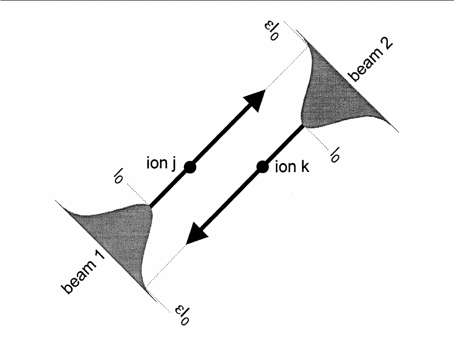
Volume 103, Number 3, May–June 1998

Journal of Research of the National Institute of Standards and Technology

Fig. 8. Scheme for differential ac Stark shifting of neighboring ions. Equal intensity counter propagating beams

1 and 2 are centered on ions j and k, respectively. A fraction

of the peak intensity I

of each beam is applied

to the other ion. This results in a differential ac Stark shift of ions j and k, allowing the possibility of individually

accessing the ions by tuning the frequency of the laser beams.

= p (a p-pulse on ion j), we find

= 0.208, and

= 1.74p. The phase shift

on ion k and the corre-

sponding phase shift on ion j must be kept track of in

subsequent operations on these ions. Generalizing this to

more than two ions becomes difficult if the laser beams

also overlap other qubit ions. This scheme places an

additional premium on laser power stability, since the

light shifts are bigger than the Rabi frequencies by 1/

1/2

for

<< 1. In addition, in both of the above schemes

employing the laser beams to differentially address

neighboring ions, one major drawback is that the posi-

tions and profiles of the laser beams must be accurately

controlled.

Many of the above differential addressing schemes

appear useful when dealing with only two ions instead

of a string of many. This leads us to seriously consider

systems where quantum logic operations are performed

on accumulators consisting of only two ions, with the

other ions located somewhere else (Sec. 5.1). A pro-

posal has also been made for transferring quantum in-

formation from one register to another by optical means

[151,278].

4.4.5 Effects of Ion Motion (Debye-Waller

Factors)

The Rabi frequency

n',n

describes the transition rate

between states ↓lnl and ↑ln'l. To realize the condi-

tional dynamics desired for quantum logic, we want

n',n

to depend on the motional quantum numbers n and n' of

a particular vibrational mode and be independent of the

state of motion of other modes. In addition, for simple

rotations on internal states, we want

n',n

to be indepen-

dent of the motional state for all modes. It is not possi-

ble, in practice, to rigorously satisfy both of these

requirements. For instance, the conventional controlled-

not gate employs two carrier pulses (steps (1a) and (1c)

in Sec. 3.3) which are intended to not depend on the

state of motion; this requires the Lamb-Dicke parameter

to be small [see Eq. (56)]. In the Raman configura-

tion,

is proportional to the difference in two wavevec-

tors and can be made negligible by using co-propagating

beams (Dk . 0). On the other hand, with single-photon

optical transitions, the Rabi frequencies depend on the

motion of all modes which have a component of motion

303

Volume 103, Number 3, May–June 1998

Journal of Research of the National Institute of Standards and Technology

along the direction of k. As discussed in Sec. 2.3, we

can take advantage of the motional dependence of the

carrier to construct a logic gate, but in this case also, the

Rabi frequency will depend on the motion in the other

modes along the direction of k or Dk. Similarly, for

sideband operations, such as step (1b) in Sec. 3.3, it will,

in general, be impossible to have

n',n

, depend on only

one mode of motion. In this section, we examine the

influence of extraneous modes on the Rabi frequencies

n',n

Transitions will generally be affected by motion in the

3L-1 spectator modes of vibration. The motion in these

other modes reduces the Rabi frequency in much the

same way as lattice vibrations affect a single emitter or

scatterer embedded in a crystal, as described by the

Debye-Waller effect [279,280]. From Eq. (36), we have

the Rabi frequency for the jth ion (assuming all modes

are in specific Fock states)

',n

j(o)

',n

k{n

pÞk

}

pÞk

†

)

{n

pÞk

(122)

j(o)

',n

pÞk

21/2(

)

((

)

where

j(o)

≡

kn'

exp(i

+ a

†

))n

l is the Rabi

frequency of the kth mode (selected for logic), in the

absence of the 3L-1 spectator modes labeled by index p

and vibrational number n

. We assume the vibrational

states of spectator modes are independently thermally

distributed with mean vibrational number n¯

(n¯

)

(1 + n¯

)

. (123)

If we average over this distribution, the mean and mean-

squared Rabi frequencies are given by

',n

j(0)

',n

pÞk

21/2(

)

(

)

j(0)

',n

pÞk

)

(n¯

+1/2)

(124)

(

',n

)

j(0)

',n

)

pÞk

)

(

)

j(0)

',n

)

pÞk

22(

)

(n¯

+1/2)

)

Ïn¯

(n¯

+1)

where we have used the Laguerre polynomial sum iden-

tities

n=0

(x)=

12z

1 2 z

n=0

(x)

2zx

12z

1 2 z

2xÏz

1 2 z

(125)

In these expressions, z < 1 and I

(

) is the zeroth

modified Bessel function with argument

The first expression in Eq. (124) shows the exponen-

tial reduction of the Rabi frequency due to motion in

modes p (Debye-Waller factor). For each mode p,we

can write (

)

(n¯

/2)=k

/2k

eff

)

l where k

eff

is the

effective k vector of the radiation and x

is the amplitude

of the component of motion parallel to k

eff

for the jth

ion. For L large, the product term on the right side of the

first expression is approximately equal to exp(2

2 k

eff

rms

)

) where x

rms

is the total rms amplitude of mo-

tion parallel to k

eff

. This is the Debye-Waller reduction

factor due to the thermal energy of the jth ion.

The second line in Eq. (124) allows us to determine

the fractional fluctuations in the Rabi frequency from

experiment to experiment

j(rms)

',n

≡

',n

= Î

pÞk

)

Ïn¯

(n¯

+1)

2 1

≈ Î

pÞk

(

)

n¯

(n¯

+ 1) . (126)

In this last approximation, the Bessel function is ex-

panded to lowest order [I

(

)=1+

/4 + ???] which is

appropriate if the 3L-1 arguments of the Bessel function

in Eq. (126) are all small compared to 1. This is ex-

pected to be the case if all modes are cooled to the

Lamb-Dicke limit [(

)

n¯

<< 1]. Eq. (126) describes

the fractional rms fluctuations in the Rabi frequency

due to thermal motion in the spectator modes of vibra-

tion.

Typically, the thermal motion is determined by initial

conditions and the reservoir is “turned off” once the

experiment begins. This is expected to be the case for

imperfect initial laser-cooling, resulting in a probability

distribution of stable Rabi frequencies with the above

mean and rms values. In this case, the Rabi frequencies

for each ion maintain a constant value during a single

run of the experiment, but deviate from the mean as

304

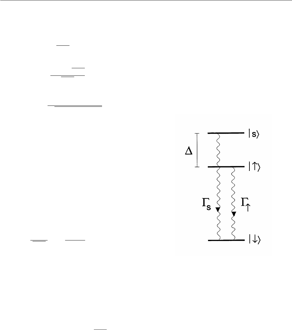
Volume 103, Number 3, May–June 1998

Journal of Research of the National Institute of Standards and Technology

indicated in Eq. (126). Stating the results in another way,

if the total number of modes is large, then the distribu-

tion of Rabi frequencies is nearly Gaussian, and the

probability that a given run of the experiment results in

a Rabi frequency which is fractionally within

of the

mean Rabi frequency

',n

)

≈ erf

Î2

pÞk

(

)

n¯

(n¯

+1)

. (127)

For example, if each of 100 spectator modes is laser-

cooled to n¯

= 0.1 and has Lamb-Dicke parameter

= 0.01, then the probability that the Rabi frequency

is within 10

of the mean value is approximately 0.23.

To see how Eq. (126) scales with the number of ions,

assume that k

eff

is aligned with the axis of a linear trap,

where the axial motion is described by L modes. If the

frequencies and amplitudes of all modes contributing to

the axial motion of ion j are assumed to be about the

same, we can write

1/2

and n¯

. n¯ where

and n¯ are the Lamb-Dicke parameter and mean occupa-

tion for the axial motion of a single (thermalized)

trapped ion. In this case, Eq. (126) becomes

j(rms)

',n

n¯(n¯+1)

1/2

. (128)

This expression indicates that a large number of ions is

beneficial because it tends to average out the effects of

motion in the (L 2 1) extraneous modes. Equation (128)

is an overestimate of the fluctuations since the L 2 1

extraneous modes will have higher frequency than the

COM mode, leading to smaller amplitudes of motion

than assumed in this crude estimate.

The Rabi frequency fluctuations discussed here trans-

late to fractional phase offsets [(

of Eq. (94)] for

each gate operation as indicated in Eqs. (124) and (126).

In practice, the mean Rabi frequency

',n

can be mea-

sured by averaging over many experiments. If we as-

sume the COM mode is used for logic, then

1/2

Therefore, for L >> 1, we cannot choose

to be too

small, or else the entangling operations for quantum

logic become too slow (Eq. (24)). To suppress the ef-

fects of Debye-Waller factor fluctuations, it is therefore

desirable to cool all modes (whose motion is parallel to

eff

) to the zero-point state.

4.4.6 Coupling to Spectator Levels

We have assumed that each time an external field is

applied to form part of a logic operation, only two quan-

tum states take part in the interaction. This assumption

is valid when any other state is far from resonance. To

explain this in a simple example, we refer to Fig. 9.

Suppose we want to drive a transition between states ↓l

to ↑l with radiation resonant with this transition. If

level ↓l is coupled to level sl with this radiation, the

wavefunction will have a small admixture of state sl

after the operation; the amplitude of state sl will be-

come larger as

becomes smaller. After a sequence of

many operations, the amplitudes of these “spectator”

states can build up and cause errors in the computation.

Fig. 9. Simplified energy level diagram for characterization of cou-

pling to, and spontaneous emission from, off resonant “spectator”

levels. We assume coherent radiation is tuned near the transition fre-

quency for the ↓lnl →↑ln'l transition (for simplicity we have

not shown the motional substructure for the ↓l and ↑l states). The

state sl is assumed to be the nearest spectator state from which

off-resonant coupling can occur.

4.4.6.1 Polarization Discrimination of Internal

States

In an array of trapped ions, two internal states of each

ion comprise a qubit of information. In addition, a third

auxiliary internal level auxl may be required (tran-

siently) for the operation of a CN gate as described in

Sec. 3.3. This state might be a particular Zeeman sub-

level of a hyperfine multiplet [17] or an optical

metastable state [1]. By employing suitable polarizations

of the driving field, particular internal state transitions

can be selected with high discrimination. Furthermore,

the Zeeman sublevels can be spectrally resolved (assum-

ing the Zeeman splitting is much larger than the Rabi

305

Volume 103, Number 3, May–June 1998

Journal of Research of the National Institute of Standards and Technology

frequency), by applying a magnetic field. This combina-

tion will help to isolate the two internal levels of interest

from other internal levels. Here, we give an example of

how polarization selection can be used to suppress cou-

pling to internal “spectator” states.

We consider the case of Ref. [17], which uses two 2s

1/2

ground state F, m

l hyperfine levels of

ions

as qubit levels. These levels are designated ↓l ≡2,2l

and ↑l ≡1,1l (Fig. 5). We also make the identification

auxl ≡2,0l. They are driven using stimulated-Raman

transitions by detuning the lasers from the

1/2

state. By

choosing the Raman beam coupling between the

1/2

and ↓l states to be

polarized and the coupling be-

tween the

1/2

and ↑l states to be p polarized, the ↓l

and ↑l states form a closed family; that is, neither the

↓l or ↑l state can be driven to other Zeeman sublev-

els. In this case, the nearest off-resonant transitions to

consider are detuned by at least the hyperfine frequency

(. 1.25 GHz in

). Similarly, by choosing the beam

coupling between the

1/2

and auxl states to be

polarized (and the coupling between the

1/2

and ↑l

states to be p polarized), the auxl level is coupled only

to the ↑l level.

4.4.6.2 Spectral Discrimination of States

Spectator states can include both motional and inter-

nal states. For example, a single CN gate uses pulses

which drive on the carrier as well as first motional

sidebands of the COM mode. Discrimination between

these two types of transitions cannot be made with

polarization selection since the relative strengths of the

matrix elements are independent of polarization. Since,

in the Lamb-Dicke limit, the carrier operation will have

a higher resonant Rabi frequency than the sideband op-

erations, the largest source of contamination may be due

to an off-resonant excitation of the carrier during the

sideband operations. The basic problem can be illus-

trated by considering the simple example illustrated in

Fig. 9. Here, we assume decay from the excited states is

negligible,

↑

= 0. We assume we want to carry out

an operation which coherently drives the ↓l ↔ ↑l

transition (resonance frequency

) and avoid the pres-

ence of any amplitude in the “spectator” state sl after

the operation. We assume radiation of frequency

is applied which couples levels ↓l and ↑l with

strength

. We assume this radiation also couples levels

↓l and sl with (resonant) strength

', but, for sim-

plicity, does not couple levels ↑l and sl. In the context

of quantum logic,

might correspond to the Rabi fre-

quency for a sideband transition and

' the Rabi fre-

quency for the carrier transition. If we take the zero of

energy in Fig. 9 to be the energy of the ↓l level, we can

write the Hamiltonian as H = H

+ H

, where

↑lk↑ +

(

)slks,

(129)

cos

[↓lk↑ + ↑lk↓]

'[↓lks + slk↓]),

where the expression for H

is equivalent to that in Eq.

(14). In the Schro¨dinger picture, we write

= C

↓

↓l +

↑

exp(2 i

t)↑l + C

exp(2 i[

]t)sl. This leads

to equations for the amplitudes

↓

= 2 i

↑

2 i

↑

= 2 i

↓

, (130)

= 2 i

2i(

↓

where

≡

and we have neglected rapidly vary-

ing terms proportional to exp(6 i(

)t) (the usual

rotating wave approximation). If we make the substitu-

tion C

= C

, the equation for C

can be written

+ iDC

= 2 i

2idt

↓

. (131)

For 

' small enough relative to 

,wecan

“adiabatically eliminate” level s, by assuming dC

dt << DC

. In this case, Eqs. (130) become

↓

. 2 i

idt

↑

+ i

(

↓

↑

= 2 i

2idt

↓

, C

. 2

2idt

↓

. (132)

The Stark shift term

≡ (

is a downward energy

shift of the ↓l state. It can be suppressed in the previ-

ous equation by including it into a shift of

. That is, by

making the substitution C

↓

= C

↓

exp(i

t) and choosing

,wefind

↓

= 2 i

↑

, C

↑

= 2 i

↓

, C

= 2

↓

. (133)

In this case, C

↓

and C

↑

are given by Eqs. (17), leading

to a the desired evolution between the ↓l and ↑l

states. Moreover, if the couplings

(and

') are turned

on and off slowly compared to 1/

(the condition of

adiabaticity), then the amplitude in state sl adiabati-

cally grows during the operation and reduces to zero

upon completion of the operation, since it is propor-

tional to

The general problem, however, is that we desire to

make all transitions as fast as possible. This means that

we cannot satisfy the adiabatic condition; therefore C

306

Volume 103, Number 3, May–June 1998

Journal of Research of the National Institute of Standards and Technology

will not be simply proportional to

' and will have some

nonzero value after

' is reduced to zero. For example,

' is turned on adiabatically, but turned off diabati-

cally, C

will have a final amplitude with magnitude



↓

. Estimates of these effects in specific con-

texts are given by Poyatos et al. [261] and James [61].

Since it should be possible to separate internal states

by relatively large frequencies and further discriminate

from internal spectator states with polarization, the most

important task will be to suppress transitions to mo-

tional spectator levels. The fundamental problem is that

in order to discriminate between carrier and sideband

transitions, the ion must be able to tell that it is moving.

If the time of the operation

is small compared to the

inverse of the frequency of the motional mode, this is

impossible. Therefore, the fundamental limit on

given approximately by 1/

COM

. To maximize computa-

tional speed, we desire to approach this condition as

closely as possible. This can be aided by using Rabi

envelopes which can suppress certain spectral compo-

nents [281,282]. Since the general problem will involve

more than one spectator level (more motional states), a

more general approach might be to apply optimal con-

trol theory [283–286].

4.4.6.3 Tailoring of Laser Fields

As discussed in the last section, the speed of an ion-

trap quantum computer will be fundamentally limited

by excitation of motional sidebands other than the de-

sired one. To see this in a specific case, the conditional

dynamics for the first CN gate described in Sec. 3.3

occurs in step (1b). That step uses a 2p pulse on 1st blue

sideband of the ↑l1l ↔auxl0l transition. To make

this step fast, we would like to increase the field inten-

sity and decrease the interaction time accordingly. How-

ever, as the pulse becomes shorter, the spectrum of the

pulse becomes wider. Eventually, the spectral width of

this pulse is larger than

so that we drive the relatively

strong and unwanted ↑l1l ↔ auxl1l carrier transi-

tion. In general, we also drive ↑l1l ↔ auxln'l tran-

sitions, where n' > 1. Most of these unwanted transitions

can be suppressed by making all terms in the expansion

in of Eq. (28) equal to zero except the term proportional

to B/z (or E/z for electric dipole transitions). In this

case, we suppress coupling to all unwanted auxl levels

except the auxl2l state whose resonant frequency is

detuned from the ↑l1l ↔ auxl0l transition by 2

Suppression of even or odd order terms in Eq. (28)

can be accomplished by appropriate positioning of

standing waves relative to the ion [40,61,287,288]. To

illustrate with an example, we first examine the transi-

tion ↓l0l ↔ ↑l1l. For simplicity, we assume single

photon electric-dipole (rather than stimulated-Raman)

transitions and consider only motion along the z direc-

tion. We want to suppress all terms in the expansion of

the field [Eq. (28)] except the E/z term. We need to

synthesize, using M separate standing wave laser beams,

a wave which has the form

E = E

m=1

sin(k

cos(

t), (134)

where k

≡ k

? zˆ, and where z = 0 corresponds to the

equilibrium position of the ion in question. The case of

M = 1 has already been suggested in various contexts to

suppress coupling to the carrier (Dn = 0) transition (see

Ref. [40] and Sec. 4.4.4 above). For M >1,wewantto

satisfy

+ C

+ ... + C

=0, n = 3,5, ... 2M 21. (135)

In this case, the next sideband spectator level which has

nonzero coupling is one where n' 2 n =2M + 1. This

transition is detuned by 2M

from the transition of

interest and the coupling is suppressed by approximately

=(k

)

compared to

1,0

0,1

Second, we consider carrier transitions ↓lnl ↔

↑lnl, where n = 0,1. With the stimulated-Raman

technique on hyperfine transitions, transitions of the

type ↓lnl ↔ ↑ln'l, n Þ n', are highly suppressed

by the use of copropagating beams. For single photon

transitions, we need to synthesize, using separate laser

beams, a wave which has the form

E = E

m=1

cos(k

cos(

t). (136)

For M >1,wewant

+ C

+ ... + C

=0,

n = 2,4, ... 2(M 2 1). (137)

In this case, the next spectator level which has nonzero

coupling is one where n' 2 n =2M. This transition is

detuned by 2M

from the carrier and the coupling is

suppressed by approximately

=(k

)

compared

1,1

0,0

. For the carrier transitions, we do not have

the problem with the remaining spectator level as noted

for the first sideband case above. On the other hand, for

logic operations which use the carrier transition (Sec.

2.3 and Ref. [174]), we do not want

to be too small,

or else the gates take to long to implement. Therefore

the suppression of the higher-order sidebands may not

be as great as in the case of logic using first sidebands.

For qubits coupled by single-photon transitions, it

may be difficult to suppress couplings to motional

307

Volume 103, Number 3, May–June 1998

Journal of Research of the National Institute of Standards and Technology

modes in the x and y directions. This will be true if we

carry out logic on a string of ions in a linear trap and use

the axial COM mode. The laser beams must be at an

angle with respect to the z axis to be able to select

particular ions. This kind of problem can be eliminated

by using the x or y COM mode for logic and making k

orthogonal to the other directions. Finally, we remark

that the use of standing waves will give rise to optical

dipole potentials which can shift the ion motional fre-

quencies. These shifts should be small, and they can be

incorporated into the definitions of the motional oscilla-

tion frequencies.

4.4.6.4 Spontaneous Emission

The internal atomic states of trapped ions, which

store quantum bits of information, must be protected

from spontaneous emission, at least for the duration of

the computation. This excludes the possibility of “error

correction,” (See Sec. 3.3) which can tolerate a certain

level of errors due to spontaneous emission. As dis-

cussed in Sec. 4.2.1, for qubit levels coupled by single

photon optical transitions, this may be accomplished by

employing long-lived energy levels which do not have an

allowed electric dipole coupling, such as metastable

electronic levels with a quadrupole or intercombination

coupling to the ground state. Although the interaction of

these states with the vacuum (causing spontaneous

emission) is reduced, their interaction with an external

field for use in quantum logic operations is also reduced.

This results in a fundamental limit on the accuracy of

each operation by roughly the ratio of the spontaneous

emission rate to the Rabi frequency

. In the case

of optical transitions,

cannot be increased indefi-

nitely, since at optical intensities beyond about 10

, the atom is quickly photoionized. This amounts to

inaccuracies due to spontaneous emission on the order

=10

2 10

[289]. Even this limit may be too

optimistic, as the two-level approximation breaks down

before photoionization occurs, and the coupling to other

electronic levels must also be considered [188,289].

This results in inaccuracies due to spontaneous emission

on the order of

=10

2 10

, depending on the par-

ticular ion used. To understand the nature of the prob-

lem, we examine a simplified system. More detailed

treatments are given in Refs. [188] and [289].

Consider the situation shown in Fig. 9. We assume

that levels ↓l and ↑l comprise the qubit states. We

want to drive coherent transitions between these two

levels but, in general, we must consider spontaneous

Raman scattering from other non resonant spectator

levels. For this approximate treatment, we will consider

only the effects of the nearest, most strongly coupled

state which is designated as state sl in the figure. For

simplicity, we assume that levels sl and ↑l are cou-

pled only to the ground state ↓l (and not each other) by

the applied radiation, and that they decay by the same

coupling process to the ground state with rates

and

↑

. To allow for different coupling processes for the sl

and ↑l states, we let

↑

and we neglect

factors

in the differences of the lifetimes (this would be valid if

the ↓l →↑l transition frequency is much larger than

). The worst case is given by considering sideband

transitions between levels ↓l and ↑l. From Sec. 2.3.1,

the resonant Rabi frequency is given by

↑,↓

1/2

s,↓

. We assume that during the operation, the ion

has a probability of about 0.5 of being in the ↓l and

↑l state. With these assumptions, the ratio

of sponta-

neous emission (from both upper levels) to Rabi fre-

quency is

↑

s,↓

, (138)

where

≡

)

, and the factors of

/2 come from the

probabilities the ion is in the ↓l or ↑l state. The most

optimistic answer is given by minimizing

with respect

which leads to

). As an approximate

“best case” we take

/2p = 25 MHz,

/2p =10

Hz,

/2p = 10 MHz,

= 0.1, giving

. 2.5 3 10

and

requiring

. 0.4

and

↑

. 10

. Therefore, weakly

allowed transitions are desirable if single photon optical

transitions are used for qubit transitions.

In the case of two-photon stimulated-Raman transi-

tions between stable electronic ground states, the ratio of

spontaneous emission rate to Rabi frequency is approxi-

mately

/(g

), where

≈

is the off-

resonant spontaneous emission rate, g is the resonant

single-photon Rabi frequency of each laser beam, and

is the detuning of the Raman beams from the excited

state (Sec. 2.3.3). This results in an inaccuracy

due

to spontaneous emission, which is independent of opti-

cal intensity. Since Raman transitions between S elec-

tronic ground states are effective only when the detun-

ing

is not much greater than the fine structure

splitting of the atom [290]; this results in an inaccuracy

due to spontaneous emission in range from about

(

)to10

(

199

), depending on the particular

ion used. Spontaneous emission from spectator elec-

tronic levels should not significantly affect this limit,

provided that their splitting from the virtual excited

state significantly exceeds

and that the single photon

resonant Rabi frequencies coupling the ground states to

the spectator levels are not much bigger than g [188].

These appear to be reasonable assumptions for most

candidate ions.

308

Volume 103, Number 3, May–June 1998

Journal of Research of the National Institute of Standards and Technology

The decohering effects of spontaneous emission can

be overcome by error correction schemes. Error correc-

tion is complicated by the fact that when spontaneous

emission occurs, the atoms may decay to states outside

the original set of computational basis states. However,

this situation can, in principle, be detected by optically

pumping the ions back to the computational basis and

applying the error correction schemes [291,292].

Spontaneous emission decoherence could, in princi-

ple, be nearly eliminated by driving single-photon tran-

sitions between ground-state-hyperfine or Zeeman lev-

els with rf or microwave radiation since spontaneous

emission from these levels is negligible. Refs. [3] and

[293] discuss this possibility, where inhomogeneous

magnetic fields couple the internal and motional states.

The speed of sideband operations is limited by the size

of the field inhomogeneity one can obtain. From Eq.

(28), we want a coupling Hamiltonian H

= 2

(B

z)z. Assume B

/z =(B

/z)

cos

and z = z

(a + a

†

) as in Sec. 2.3.1. For resonance at the

first red sideband (

), H

is given by Eq. (27)

with

= 2

(B

/z)

/(4

). If we take

= 10 nm, then to achieve

/2p = 1 MHz, we require

(B

/z)

. 290 T cm

; a difficult task. Moreover, it

would be difficult to address selected ions because of

the long wavelength of the radiation relative to typical

ion spacings (see also Sec. 5.3).

4.4.7 Mode Cross Coupling During Logic

Operations

In the preceding sections, we have assumed that when

transitions are driven between ↓l

n

l and ↑l

n

involving a single mode of motion k, the other 3L-1

spectator modes of motion are not affected because

coupling to them is nonresonant. However, when the

sum or difference frequency of two or more spectator

modes is near the frequency of the desired mode-k tran-

sition (

n

2 n

), higher order couplings can entan-

gle the ↓l

n

l and ↑l

n

l states with the spectator

mode states.

Equation (33) describes the general interaction

Hamiltonian between the internal levels of ion j and all

3L modes of motion. By expanding the exponential in

Eq. (33) to all orders, we find

l=1

†

)

3 e

i(b

)

2i(

)

+ h.c.

, (139)

where

' =

exp[2

(

)

]. This equation describes

the processes of each mode l gaining or losing (b

2 d

)

vibrational quanta, accompanied by the raising or lower-

ing of the internal electronic levels of ion j. In general,

we must account for all terms in Eq. (139) which do not

vary rapidly in time, or terms in which the resonance

condition is nearly met: S

2 d

)

' 2

). Although detailed treatment of this problem is be-

yond our intent, a couple of comments may be made.

In general, we must account for all the terms in Eq.

(139) which cause significant errors in the overall com-

putation we are trying to carry out. For two or more

trapped ions, some combination of modes will nearly

always satisfy the resonance condition. However, this

may occur only for high orders of b

and d

, and if the

Lamb-Dicke criterion is met, the contributions are van-

ishingly small. The terms that will cause problems are

the ones that are close to satisfying the resonance condi-

tion and are relatively low order in b

and d

.Ifthe

Lamb-Dicke criterion is satisfied, it will always be pos-

sible to avoid these spurious couplings, but it may be at

the expense of making the Rabi frequency so small (in

order to avoid coupling to relatively nearby off-resonant

terms) that the operations will become too slow.

To understand this problem in the context of a simple

example, we assume that a cross-mode coupling of this

type occurs when two modes, p and q, have frequencies

which satisfy the condition n

2 n

. 0, or 6

corresponding to possible extraneous mode coupling on

the carrier, first blue sideband, or first red sideband of

the logic operations (assumed to utilize mode k). This

additional resonance condition yields, to lowest order in

the Lamb-Dicke parameters, the effective Hamiltonian

1+i

+ a

†

)

†

)

i(n

2i(

)

+ h.c., (140)

where the resonance conditions are given by

≡

=0,+

,or2

. A specific example is relevant to

the NIST single

ion experiments. Here, mode k was

the x oscillation, and modes p and q are identified with

the z and y oscillations of the single ion in the trap. In

this experiment

= k ? xˆx

= k ? yˆy

= k ? zˆz

and

. (The frequency relationship

is a consequence of Maxwell’s equations

for a quadrupole rf trap in the absence of static poten-

tials applied to the electrodes [211].) We assume that the

desired transition is the first blue sideband of mode

). In this case, the resonant part of Eq. (140)

becomes

†

+ O(

)

+ h.c.

(141)

309

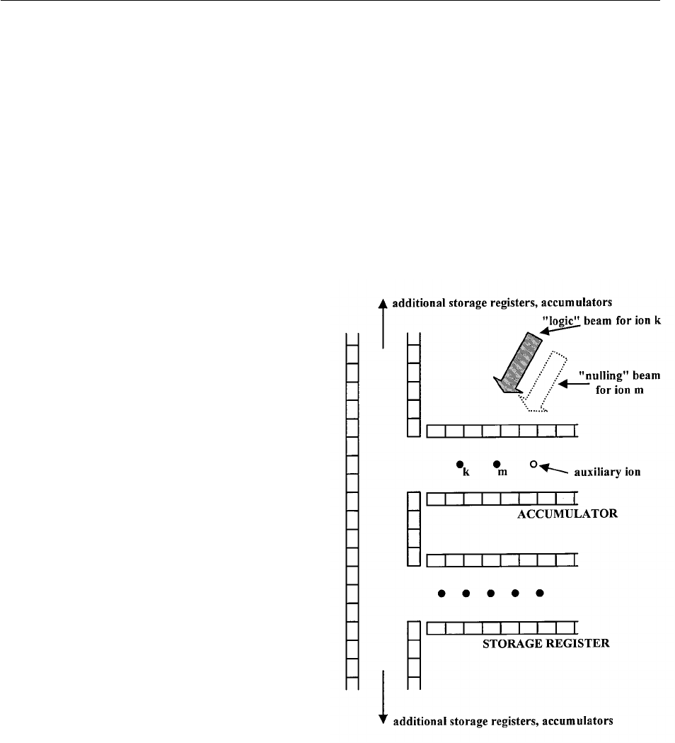
Volume 103, Number 3, May–June 1998

Journal of Research of the National Institute of Standards and Technology

The term proportional to a

†

is the desired anti-Jaynes-

Cummings operator, and the term proportional to a

†

can entangle the internal state with the other spectator

modes (z and y), leading to errors.

For logic operations on a string of ions in a linear

trap, we will assume that all other mode frequencies are

higher. With the use of stimulated-Raman transitions,

we can make Dkizˆ and restrict our attention to spectator

modes along the z axis. Nevertheless, as L becomes

large, nearby resonances of the type shown in Eq. (140)

will become harder to avoid. These coupling terms al-

ways scale as products of Lamb-Dicke parameters. Thus

if the spectator mode Lamb-Dicke parameters are small

enough, or if at least one Lamb-Dicke parameter is ap-

proximately zero, the higher order unwanted resonances

may be sufficiently suppressed. Furthermore, if the

spectator modes are cooled to near the zero-point energy

(knˆl << 1), then any couplings in Eq. (140) with powers

of the annihilation operator a

will be absent most of the

time. Hence, in large registers, it will probably be im-

portant to cool all modes to near the zero-point energy.

5. Variations

5.1 Few-Ion Accumulators

Many of the problems anticipated above, such as un-

wanted coupling to adjacent ions or spectator modes,

will be aggravated by a large number of ion qubits in a

single ion trap “register.” Moreover, implementation of

quantum error correction schemes will require highly

parallel processing [294]. Therefore, a multiplexing

scheme for ion qubit registers is desirable. One possibil-

ity is to perform all logic in minimal accumulators

which hold one or two ions at a time [65]. Ions would be

shuffled around in a “super-register” and into and out of

(multiple) accumulators which are well shielded from

the other ions. The shuffling could be accomplished

with interconnected linear traps with segmented elec-

trodes as shown schematically in Fig. 10; construction

of such traps appears to be possible with the use of

lithographic techniques [295]. Single-bit rotations on

the mth ion would be accomplished by moving that ion

into an accumulator. Logic operations between ions m

and k would be accomplished by first moving these ions

into an accumulator. An accumulator could also hold a

second species of ion (say Mg

) which could be used to

provide laser cooling to the n =0l state of the motional

mode used for the logic operations, if necessary. There-

fore, for logic operations, an accumulator would hold

two computational ions and the auxiliary ion. This

scheme should make it easier to select ions with laser

beams because it should be possible to address one ion

while nulling the laser intensity on the other ion, even

with very high trap frequencies (see Sec. 4.4.4). The

very small number of logic ions in an accumulator (1 or

2) would make extraneous mode coupling much easier

to avoid. The main disadvantage appears to be that com-

putational speed is reduced because of the time required

to shuffle ions in and out of the accumulator and provide

laser cooling with the auxiliary ion, if required. How-

ever, energy shifts of the ion’s internal structure, due to

the electric fields required to move the ion, need not be

severe. For example, to move a

from rest to a

location 1 cm away (and back to rest) in 1 ms would

require a field of less than 50 V/cm. Electric fields of

this order should give negligible phase shifts in qubits

based on hyperfine structure (Sec. 4.2.3). The accompa-

nying phase shift caused by time dilation for a transition

Fig. 10. Schematic diagram of an ion trap “super-register” containing

few-ion accumulators in which logic operations are performed. We

assume the trap is generically equivalent to the linear trap of Fig. 1.

The rods of the trap in Fig. 1 are replaced by segmented electrodes in

which adjacent segments are at the same rf potential but where the

segments support different static potentials. This allows ions to be

selectively moved around an in and out of ion accumulators. In the

accumulator shown a logic operation between ions k and m is indi-

cated. The configuration of the laser beams is chosen to null the

intensity on ion m while performing an operation on ion k. The beams

must be reconfigured to perform an operation on ion m while leaving

ion k unaffected. The auxiliary ion may be required to perform laser

cooling each time new logic ions are moved into the accumulator.

310

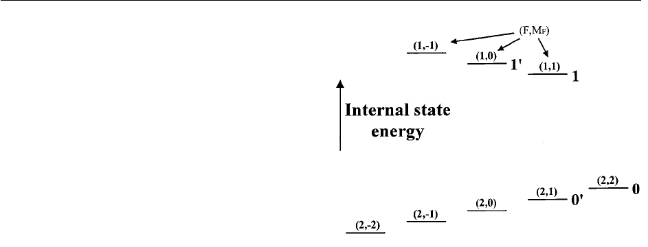
Volume 103, Number 3, May–June 1998

Journal of Research of the National Institute of Standards and Technology

frequency

/2p = 1.25 GHz (hyperfine structure in

) would be less than 1 mrad.

5.2 Multiplexing With Internal States

In principle, it should be possible to multiplex quan-

tum information into all 3L modes of ion motion. This

will probably be useful in experiments which use a

small number of ions. However, because of the higher

potential for decoherence of motional modes, it might

prove more useful to multiplex quantum information in

multiple internal states. This would give more work

space with a smaller number of ions. Quantum logic

within multiple internal states would most likely follow

the ideas of NMR quantum computing [165,166]. A

simple example is given by the eight ground state hyper-

fine levels in

which can be labeled like states of

three coupled spin-

/2 particles 

l where

[ {0,1}. For instance, a Toffoli gate [140] is realized

by driving a p pulse on the F,M

l = 2,2l →1,1l

transition in the ground state hyperfine manifold of

if we label the states 2,2l ≡1,1,0l and 1,1l ≡1,1,1l,

in the notation F,M

l ≡

l. Technically, the

readout of specific internal quantum states would be

more complicated since the methods employed in the

experiments so far distinguish between only two possi-

bilities, seeing fluorescence or not seeing fluorescence,

on any given ion. However, by appropriate mappings,

superpositions of any two internal states could be

mapped onto two states of “readout” ions and the detec-

tion accomplished as described above. To multiplex in-

formation into internal states, we need a way to map

qubits from any ion into the internal levels of other ions.

To give a specific example of how this can be accom-

plished, we consider the case of

where we might

wish to multiplex into the F,M

l = 2,2l, 1,1l, 2,1l,

and 1,0l states shown in Fig. 11. This figure is essen-

tially the same as Fig. 5, but for simplicity of notation,

we label these hyperfine states as 0l, 1l, 0'l,and1'l

respectively. We want to accomplish the transformation

u0l

u1l

u0l

+du1l

u1l

➾

u0l

u1l

u0'l

+du1'l

u0l

(142)

between ions A and B. This can be realized with the

transformation

= C

A',B

? C

A,B

? C

B,A'

? C

B,A

A,1,0'

, (143)

where the operator P

A,1,0'

denotes a p transition between

the states u1l

and u0'l

on ion A and the operators C

c,t

are defined in Sec. 3.3. For example, C

A',B

denotes a

controlled-not operation with the u0'l

and u1'l

states

acting as the control bit states and the u0l

and u1l

states

acting as the target bit states.

5.3. High-Z Hyperfine Transitions

The possibility of using highly charged ions as qubits

poses some interesting possibilities. For simplicity, we

consider using hyperfine states in high-Z hydrogenic

ions as qubit levels where Z is the nuclear charge.

More complicated high-Z ions appear to show similar

features. If Z is high enough, hyperfine transitions occur

in the optical region of the spectrum. Therefore, the

required high field gradients necessary for quantum

logic would be provided by the laser fields used to drive

the hyperfine transitions. The potential advantages

are: (1) Off-resonant spontaneous scattering, which is a

source of decoherence in other cases (Refs. [188], [289],

and Sec. 4.4.6.4), is essentially eliminated since the first

excited 2p level is at much higher energy above the

ground state. (2) The trap binding of high-Z hydrogenic

ions can typically be stronger that singly-ionized atoms,

thereby increasing motional frequencies and reducing

the time of fundamental operations. The disadvantages

are (1) High-Z ions are hard to produce. (2) The life-

times of the upper hyperfine states are short enough that

Fig. 11. Hyperfine levels of the 2s

1/2

ground state of

in a weak

magnetic field (not to scale). The energy levels are designated by

horizontal lines. Above the lines, the levels are represented by atomic

physics labels (F,M

) where F is the total angular momentum and M

is the projection of the angular momentum along the magnetic field

axis. The separation of Zeeman substates in the different F manifolds

is approximately equal to 0.7 3 10

Hz where B

is expressed in

teslas. The separation of the F = 1 and F = 2 manifolds is approxi-

mately 1.25 GHz at B

= 0. For simplicity of notation, in Sec. 5.2, we

make the identifications F,M

l = 2,2l ≡0l, 1,1l ≡1l, 2,1l ≡

0'l, 1,0l ≡1'l.

311

Volume 103, Number 3, May–June 1998

Journal of Research of the National Institute of Standards and Technology

spontaneous emission decoherence from these states

cannot be neglected. (3) Detection of internal states may

be difficult.

The ion production problem is not intractable; for

example, recent storage ring measurements have been

able to determine the transition wavelengths and life-

times of hydrogenic

209

82+

[296] and

165

66+

[297].

Effort in some laboratories is directed to transferring

similar high-Z ions to low energy ion traps. The hyper-

fine frequency of a hydrogenic ion can be estimated to

hfs

/2p ≈2.54310

Fug

u Hz, where F and F-1 are

the values of angular momentum in the hyperfine states

and g

is the nuclear g-factor (

, m

= nuclear

magneton, I = nuclear spin) [298]. The spontaneous

decay rate from the excited state is estimated to be

rad

=1/

rad

≈ 1.01310

–42

/(2F

+1)] (

hfs

/2p)

–1

where the term in square brackets [298] depends on

matrix elements and is on the order of 1. For example,

the hyperfine transition in

209

82+

has a wavelength of

244 nm and the upper level decays with a lifetime of

351 ms [296]. For

165

66+

, the transition wavelength is

573 nm and the decay time is 2 to 3 ms [297]. These

experimental numbers agree roughly with the formulas

above. These wavelengths are reasonable for quantum

logic, but the lifetimes are somewhat short. However

since the lifetime scales as 1/Z

, it might be possible to

use lower Z, longer wavelength transitions. The readout

of the qubits appears difficult, because coupling to a

higher electronic level and observing fluorescence is

impractical due to the short wavelengths involved. In

principle, however, the qubit information from these

ions could be transferred to other ions whose states are

easier to read, perhaps using small accumulators as

described in the previous section and in Sec. 4.3.

6. Other Applications

6.1. Quantum Correlations

In a classic Paper, Einstein, Podolski, and Rosen

(EPR)[299] argued that quantum mechanics provides an

incomplete description of physical reality and specu-

lated that it might be an approximation to some theory

which would provide a complete description. Today

such theories, which supplement quantum mechanics

with additional, as-yet unobserved parameters, are

called hidden-variables theories. If such a theory obeys

some physically reasonable conditions forbidding action

at a distance, it is called a “local hidden-variables

theory.”

Simple quantum logic gates performed on small

numbers of trapped ions can lead to interesting experi-

ments which may shed light on the viability of local

hidden-variables theories. For example, as described by

Cirac and Zoller [1] and Sec. 3.4, using controlled-not

gates, we can generate the state

Ï2

(u↓l

u↓l

u↑l

). (144)

In the context of EPR, this is called a Bell state. Accord-

ing to Bell’s theorem [300], such a state allows us to

distinguish between quantum mechanics and all local

hidden-variables theories. If the states of the two en-

tangled particles are detected outside of each other’s

light cones, then, for particular sets of measurements,

we may derive inequalities which all local hidden-

variables theories must obey, but which quantum

mechanics violates. The experiments performed by

Clauser and Shimony [301] and Aspect et al. [302]

provide strong evidence against local hidden-variables

theories. Their work used polarization measurements on

entangled pairs of photons. In their experiments, the

detection of the photons’ polarization states occurred

outside each others’ light cones. Thus, the measurement

on one photon could not possibly have affected the other

measurement, which closed possible “loopholes” in the

proof of quantum mechanics over other explanations.

However, some loopholes still remain open. Since the

photon detection in the Aspect, et al. experiments was

not 100 % efficient, the group had to make assumptions

that the photons they measured were a “fair” sample of

the whole population of events. Thus, their experiments

do not rule out the (seemingly implausible) possibility

of local hidden-variables theories in which the hidden

variables cause some sub-ensemble of the photon

pairs to preferentially interact with the measurement

apparatus.

In the system of two ions, we may detect the state of

either ion with nearly 100 % efficiency through the use

of “electron shelving” (Sec. 2.2.1). On the contrary, it

will be difficult to perform measurements on two ions

outside each other’s light cone. Such a measurement

would require separating the ions by a distance larger

than the speed of light times the measurement time or

transferring quantum information over large distances

[151]. (In principle, the ions could be first entangled and

then placed in different traps which could be separated

by large distances before measurements were per-

formed.) Nonetheless, an experiment with two trapped

ions could be viewed as complementary: the photon

experiments definitively close loopholes of causality,

and the ion experiments could close loopholes due

to detection inefficiency. Such experiments have the

additional appeal of studying EPR on massive particles

[303]. EPR states of atoms have recently been created

in an atomic beam using the methods of cavity QED

[304]; if detection efficiency can be improved, these

experiments could also close loopholes due to detection

inefficiency. Moreover, even though measurements of

quantum correlations between entangled ions cannot be

312

Volume 103, Number 3, May–June 1998

Journal of Research of the National Institute of Standards and Technology

easily performed outside each other’s light cone, one

can argue strongly that the ions cannot transfer infor-

mation by any known mechanism. Therefore, if the

observed correlations violate Bell’s inequalities, the

correlations are established by some new force of nature

or are, in fact, inherent in the structure of quantum

mechanics.

An intriguing possibility for ions is the possibility of

making “GHZ states” [54,305,306]. For three ions, the

GHZ state is

Ï2

(u↓l

u↓l

u↑l

). (145)

For such a state, a single measurement can distinguish

between the predictions of quantum mechanics and

those of any local hidden-variables theory [54,305].

Aside from this, Bell states, GHZ states, and

Schro¨dinger-cat states are highly entangled, and are thus

of inherent interest for the study of uniquely quantum

behavior. As the experiments improve, it will be interest-

ing to push the size of entangled states to be as large as

possible. The question is not whether we can make states

which have the attributes of Schro¨dinger cats, but how

big can we make the cats? Certain theories which

address the measurement problem will be amenable to

experimental tests, for example, quantitative limits on

spontaneous wavefunction collapse theories [307,308]

can be established. The isolation from the environment

exhibited by trapped ions, coupled with the control

possible over their quantum state and high detection

efficiency make them an interesting laboratory for the

study of fundamental issues in quantum mechanics.

6.2. Simulations

The nonlinearities with respect to motional raising

and lowering operators inherent in the coupling

Hamiltonians of Eqs. (14), (37) and (48) can lead to a

rich variety of dynamics between the ion motion and

internal levels. Some of these dynamics for a single ion

have been discussed in Sec. 3.2. An interesting system

which can be simulated with these couplings is a

“phonon maser” which provides vibrational ampli-

fication by stimulated emission ofˇ radiation [309]. This

would be an analog of the micromaser with some

interesting differences such as the effects of recoil in the

pumping process.

The Hamiltonians of Eqs. (14), (37) and (48) for a

single ion can be consolidated into the general interac-

tion Hamiltonian

[k ? x–dt+

]

+h.c., (146)

where d =

–

, where we have used the rotating-wave

approximation, and where we have neglected phase

factors of the field. The parameter

is equal to 1 when

internal state transitions are involved and

= 0 when the

internal state is unchanged. In Eq. (146), k is the

wavevector of the field for single photon transitions or

k → k

– k

when stimulated-Raman transitions are

used. Similarly,

is the frequency of the applied field

for single-photon transitions and

→

–

when

stimulated-Raman transitions are used. In an interaction

picture of the ion’s motion, this Hamiltonian becomes

–i(dt–

)

j=x,y,z

exp(i[

–i

†

)+h.c.

, (147)

where

≡ k?xˆx

, a

is the lowering operator for the

x motion of frequency

, etc. Now, assume that

small enough, and that, in general,

,and

are incommensurate, so that we can excite only one

spectral component of the possible transitions induced

by this interaction. For a particular resonance condition

=–

–

, and in the Lamb-Dicke limit,

we find

≈

j=x,y,z

)

+(1–

)

†

)

+h.c. , (148)

the two mode case where

= 0 is considered by

Drobny´ and Hladky´ [310], and in a different excitation

scheme in Ref. [110]. If the Lamb-Dicke limit is not

rigorously satisfied, we must consider higher order non-

linear corrections to this expression; specific examples

are discussed in Refs. [28] and [110]. These nonlinear

terms are the origin of the high-order corrections to the

Rabi frequencies (Eq. (18)). The case of carrier, and first

red and blue sidebands on internal state transitions (e.g.,

=1,

= 0,

=0,61) are used extensively for

quantum logic and generation of nonclassical motional

states and are discussed above. The case

=0,

= 0, u

u = 1 has been used to create coherent

[21] and Schro¨dinger cat [47] states of motion and is

discussed in Sec. 3.1. The case

=0,

= 0,

u = 2 has been used to create squeezed states; this is

discussed in Ref. [21]. A realization of the Hamiltonian

~ S

†

)

+h.c. (

=1,

= 0,

= –2) has

been reported by Leibfried, et al. [132]. This is similar

to the case of two-photon excitation in cavity QED

analyzed by Buck and Sukumar [311] and Knight [312].

313

Volume 103, Number 3, May–June 1998

Journal of Research of the National Institute of Standards and Technology

Interactions proportional to S

†

+h.c., S

†

+h.c.,

and a

†

+h.c. might be used to generate the maximally

entangled state of Eq. (60) without the need to address

individual ions [194]. An example of an interesting new

case would perhaps be the realization of three-phonon

downconversion (e.g.,

=0,

=3,

=–1,

= 0).

This case is analogous to three-photon downconversion

in quantum optics (see Refs. [110],[313], and references

therein). Here, it corresponds to driving a two-mode

resonance using stimulated-Raman transitions where

–

–3

. A suggestion to realize a

Hamiltonian ~a

†

+h.c. (

=0,

=2,

=–1)

is discussed by Agarwal and Banerji [314]. Clearly, a

large number of possibilities could, in principle, be

realized just for a single ion; moreover, the number of

possibilities increases dramatically if we consider all

modes of motion for multiple trapped ions. The only

limitation on how high u

u in Eq. (148) can be is that

be chosen sufficiently small that couplings to other

(unwanted) resonances are avoided. This will require

that decoherence be small enough to see the desired

dynamical behavior before coherence is lost.

Various forms of interactions which satisfy the

requirements of quantum nondemolition (QND) mea-

surements [20,25,315] of ion motion or quantum

feedback [316] can be extracted from Eq. (148). QND

experiments employing dispersive interactions are

considered by Retamal and Zagury [36]. These schemes

rely on measuring the ion’s internal state however,

which almost always involves recoil heating, thereby

destroying the state we wish to preserve. This could be

circumvented by coupling the ion’s motion to a cavity

field which then serves as the probe [317].

6.2.1 Mach-Zehnder Boson Interferometer With

Entangled States

Realization of the various Hamiltonians indicated in

Eq. (148) can lead to simulation of various devices of

practical interest. As an example, consider a Mach-

Zehnder interferometer which acts on two modes of

oscillation of a single trapped ion; to be specific, we will

consider the x and y modes of motion. The analogy with

a Mach-Zehnder interferometer for bosons is that

the two input modes to the boson interferometer are

replaced by the x and y modes of ion oscillation. The

(50/50) beamsplitters in the boson interferometer are

replaced by an operator B

= exp[6ip(a

†

/4]

[193,318,319]. This operator can be realized by

applying the interaction in Eq. (148) with

=0, and

=–

= 1 for a time given by

t=p/4. A

differential phase shift between the two arms of the

interferometer can be simulated by shifting the relative

phases of the fields in Eq. (148) between successive of

applications B

. In a particle (e.g., boson) interfero-

meter, one typically measures the number of particles in

either one or both output modes. In a single ion experi-

ment, we have only one convenient observable, the inter-

nal state of the ion (either u↓l or u↑l. Nevertheless, we

can characterize the action of the phonon interferometer

by repeating the experiment many times and measuring

the density matrix of the output state [132].

It will be most interesting to characterize the action of

the interferometer for various nonclassical input states.

One example is the two-mode Fock state un

[195]. This state could be prepared by applying the

techniques described in Sec. 3.2 sequentially to the ion’s

x and y modes. This state is interesting because it has

been shown that one could approach the Heisenberg

uncertainty limit in a Mach-Zehnder interferometer by

measuring the distribution of bosons in the output

modes [195,196,197]. An alternative technique for

studying the action of a beamsplitter on the two-mode

Fock states has been suggested by Gou and Knight [23]

when

. Here, a beamsplitter could be simulated

by first preparing un

along two orthogonal axes

and then probing along two other axes (x' and y') which

are rotated (in the xy plane) with respect to the first. This

technique could also be used to analyze, for example, the

(u0l

u2l

+ u2l

u0l

)/Ï2 state from an initially pre-

pared u1l

u1l

state [23].

Another interesting state to consider for the phonon

interferometer is the (uNl

u0l

+(u0l

uNl

)/2

1/2

state

(which is the desired state after the first beam splitter).

This state has been shown to yield exactly the

Heisenberg uncertainty limit for an interferometer for

any value of N [194], if after the second beamsplitter,

we measure the number of particles N(x)inthex output

port. The result of this measurement is assigned the

value (–1)

N(x)

. This state could be prepared from the

u↓lu0l

u0l

state by the following two steps:

(1) Apply a p/2 pulse on the Nth blue sideband of mode

x [

=1,

=–N,

= 0 in Eq. (148)]; this creates the

state (u↓lu0l

+u↑luNl

)u0l

1/2

(2) Apply a p pulse on the Nth blue sideband of mode

y [

=1,

=–N in Eq. (148)]; this creates the

state u↑l(uNl

u0l

+u0l

uNl

)/2

1/2

After the second beamsplitter, we have a state which can

be written as

final

= u↑l

= 0

uN–n

)

. (149)

314

Volume 103, Number 3, May–June 1998

Journal of Research of the National Institute of Standards and Technology

In principle, we would like to measure

, record the

value N(x), and assign the value (–1)

N(x)

. Effectively,

this assignment can be accomplished if we can find an

interaction M which provides the mapping

final

= u↑l

even

)

uN–n

)

+ u↓l

odd

)

uN–n

)

. (150)

After this mapping, we need only measure the internal

state; if the ion is found in the u↑l state we assign the

value +1 to the measurement; if the ion is found in

the u↓lstate, we assign the value –1. The mapping

M can be achieved by applying radiation with k i xˆ

at the carrier frequency (

=1,

= 0) and insuring

n,n

t =2pm6n

p where m is an integer. From Eq. (18),

we have

t ≈

–

1–n

– n

. (151)

Therefore, if we make

exp(–

/2)t=2mp and

(1+

/4=(2m

–1

) we achieve the desired mapping as

long as the contribution to the phase from the term

proportional to n

in this equation is small compared to

p. Therefore we require m>>N

/8 or, equivalently,

<<2/N.

One final example of a two-mode phonon interfero-

meter which directly yields Heisenberg 1/N phase sensi-

tivity is a “beamsplitter” which creates the state

(u↓lu0l

uNl

+u↑luNl

u0l

)/Ï2. This state can be cre-

ated by starting with an initial (u↓l+u↑l)uN/2l

uN/2l

Ï2 dual Fock state (Sec. 3.2). Next, we apply N/2

p-pulses alternating between the two interaction

Hamiltonians H

†

+h.c.)and

†

+h.c.) which can be realized in the

Lamb-Dicke regime. In this way, the state of motion of

the ion is stepped through

u↓lu

+u↑lu

→

u↑lu

+1l

–1l

+u↓lu

–1l

+1l

→

u↓lu

+2l

–2l

+u↑lu

–2l

+2l

→

. (152)

u↓luNl

u0l

+u↑lu0l

uNl

where, in this example, we assume N/2 is even. The

interactions H

and H

follow from Eq. (148) with e=1,

=–1,

= 1,

= 0 and e=1,

=1,

= –1,

=0,

respectively. The kth pulse has Rabi frequency

[(N/2+k)(N/2–k+1)]

1/2

in the Lamb-Dicke re-

gime. After a relative phase is accumulated in the two

“paths” of the interferometer (simulated by adjusting

the phase of the laser pulses as discussed above), we

reverse the above steps and apply a final “p/2” pulse on

the carrier. Upon measuring the probability of occu-

pation in state u↓l or u↑l, the interference fringes exhibit

1/N phase sensitivity.

If the Lamb-Dicke criterion is not satisfied, the two

components of the wavefunction superposition may

experience different Rabi frequencies during each pulse,

leading to undesired evolution. The exact Rabi frequen-

cies of the two components of the wavefunction upon

application of the kth pulse (interaction H

or H

) follow

from Eq. (18):

–1/2(

)

N/2+k–1

(

) L

N/2–k

(

)

Ï(N/2+k)(N/2–k+1)

(153)

–1/2(

)

N/2+k–1

(

) L

N/2–k

(

)

Ï(N/2+k)(N/2–k+1)

where

is the Rabi frequency between states

uN/2+k –1l

|N/2–k+1l

and uN/2+kl

|N/2–kl

and

is the Rabi frequency between states uN/2–k+1l

|N/

2+k –1l

and uN/2–kl

|N/2+kl

. The only differences

between

and

are the arguments of the associated

Laguerre polynomials. Thus, as long as

, the

system will evolve as in Eq. (152), even when the Lamb-

Dicke criterion is not satisfied.

6.2.2 Squeezed-Spin States

As an example which demonstrates the advantages of

using entangled states in spectroscopy, we discuss the

following simple experiment which can be carried out

on a single ion. Let us suppose we are interested in

measuring, with maximum signal-to-noise ratio, the

Zeeman frequency between states of a J = 1 manifold in

an atom. To be specific, consider that we are interested

in measuring the Zeeman frequency of the DM

= 61

transitions in the

1/2

(F=1) ground-state hyperfine

multiplet of a

ion (Figs. 5 and 11). This manifold

is composed of the three levels uF,M

l [ {u1,0,l,

u1,61l}. We will assume that the applied field is small

enough that the frequency of the u1,–1l → u1,0l transi-

tion is equal to the frequency of the u1,0l → u1,1l transi-

tion. A straightforward way to measure the Zeeman

frequency would be to prepare the atom in the u1,1l

315

Volume 103, Number 3, May–June 1998

Journal of Research of the National Institute of Standards and Technology

(or u1,–1l state, drive the Zeeman transition (using the

Ramsey method), and then measure J

. We will assume

this detection can be accomplished with 100 % detec-

tion efficiency, so the noise in the measurement is

limited by the quantum statistics in the measurement

process [100]. After many measurements, requiring a

total averaging time

, a certain precision in the Zeeman

frequency would be obtained. However an alternative

measurement strategy, described below, would require

an averaging time

/2 to reach the same measurement

precision.

The basic idea is outlined in Ref. [9]; for J =1,itis

equivalent to the more general technique described by

[194]. We prepare the atom in the state

(0) = u1,0l and

then apply the Ramsey fields. Subsequently, we measure

the probability of the ion to remain in the u1,0l state.

(This measurement scheme has been used in the exper-

iments of Abdullah et al. [320]; the noise in these exper-

iments, however, was not limited by projection noise.)

This measurement is equivalent to measuring the opera-

tor

–J

, where

is the identity operator, and therefore

equivalent to measuring the operator J

, as discussed by

Wineland, et al. [9], or the operator P

, as discussed

by Bollinger, et al. [194]. After application of the first

Ramsey pulse to the u1,0l state, the ion is in the state

(u1,1> + u1,–1l)/Ï2; this is equivalent to the maximally

entangled state of Eq. (60) which could be formed by

two spin-1/2 particles. As described in Sec. 3.3, we

would expect the time required to reach a certain

measurement precision to be reduced by a factor of

2(L = 2) over the case of uncorrelated particles, repre-

sented by starting the ion in the state

(0) = u1,1l or

u1,–1l state and finally measuring J

We could carry out this experiment in the following

way. We first optically pump the ion to the u2,2l hyper-

fine state. We then apply two successive p pulses which

carry out the transformations u2,2l → u2,1l → u1,0l with

stimulated-Raman transitions. We then perform Ramsey

spectroscopy on the u1,0l state. We can measure the

probability of subsequently finding the atom in the u1,0l

state by first reversing the order of the two p pulses and

then measuring the probability of finding the ion in the

u2,2l state.

6.3 Mass Spectroscopy and NMR at the Single

Quantum Level

Quantum logic operations may be useful in precision

measurements other than spectroscopy (Sec. 3.4). For

example, Ref. [48] discusses a method to measure

cyclotron resonance frequencies of single ions at the

quantum level; this technique essentially employs quan-

tum logic to distinguish between motional quantum

states. This capability would provide mass spectroscopy

at such low energies that anharmonic shifts (electric

potential and relativistic) would be very small. (At

present, however, high-resolution mass spectrometry

experiments are limited by other effects such as mag-

netic field drifts [77,78,79].) In mass spectroscopy, the

basic problem is to measure a “test” ion’s cyclotron

frequency and compare it to the cyclotron frequency of

a “measurement” ion (in the same magnetic field) which

serves as the transfer standard.

One idea [48] is to store two ions in separate Penning

traps which are stacked along their symmetry axis and

share a common endcap and a common, axial magnetic

field. The axial frequencies of the ions are adjusted to be

the same, in which case the axial harmonic oscillators

are coupled through the charge in the common endcap.

The technique might work as follows: The axial motion

of the “measurement” ion (for example,

)isfirst

laser cooled to the n = 0 level. When the ions’ axial

modes are resonantly coupled, this cooling can be trans-

ferred to the test ion’s axial motion; if the coupling is left

on for a certain amount of time, the energies in the ions’

axial oscillations are exchanged. Subsequently, the

ion’s axial oscillation is recooled so that both ions are

cooled to the zero-point energy. This axial cooling is

then transferred to the test ion’s cyclotron mode by

parametric coupling, after which the axial motion of

the measurement ion must be recooled to the zero-point

energy. An external field is then applied to weakly

excite the test ion’s cyclotron motion. When the ampli-

tude of this field is adjusted appropriately and the

resonance condition is met, the n =0ton = 1 transition

in the test ion is driven with high probability. The steps

above are then reversed so that if the test ion’s cyclotron

motion was excited to the n = 1 level, the

ion’s axial

motion is now in the n = 1 level. When the resonance

condition for the test ion’s cyclotron frequency is not

met, the

ion’s motion remains in the n = 0 level.

Discrimination between the n = 0 and n = 1 axial level is

then performed using quantum logic operations applied

to the

ion as discussed in Sec. 3. For example, after

the steps above, an axial red sideband p pulse will excite

a u↓l → u↑l transition in the

ion conditioned on

whether or not the

ion’s axial mode was in the

n =0orn = 1 state. The test ion’s cyclotron frequency

can be referenced to a spin flip frequency in

(either

electron or nuclear) which then acts as a transfer

standard. Finally, by performing a cyclotron resonance

measurement on a second test ion in the same fashion

we can find the ratio of the two test ions’ cyclotron

frequencies and therefore derive their mass ratio.

Ref. [48] also suggested that these ideas could be

applied to measure magnetic moments of test ions. In

this section, we describe a variation on the method dis-

cussed there. The basic idea is to perform NMR on an

––

316

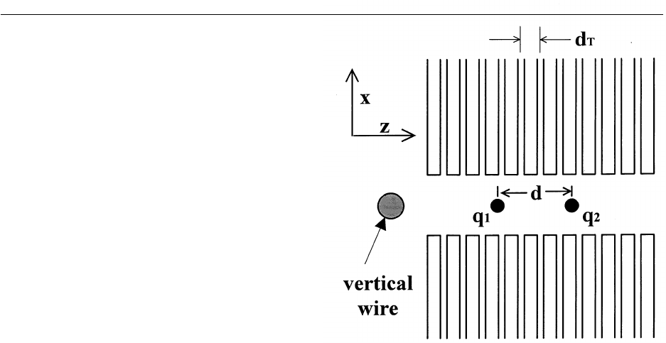
Volume 103, Number 3, May–June 1998

Journal of Research of the National Institute of Standards and Technology

unknown magnetic moment (the test ion) at the single

spin level. Using quantum logic operations, the spin flip

is detected in a measurement ion to which the test ion is

coupled. We will describe the ideas in the context of a

specific example; but the techniques are easily general-

ized to measuring the magnetic moments of other ions.

Suppose we want to measure the ratio of proton and

antiproton magnetic moment. Such a measurement is of

high current interest and can provide a second test of

CPT on baryons in addition to the precise mass com-

parisons already performed [79]. Precision measure-

ments of the magnetic moment ratios coupled with the

mass ratios should test much of the same physics in the

context of CPT as precision spectroscopy of antihydro-

gen [321]. A measurement scheme for the proton/

antiproton moment ratio has been suggested previously

by Quint and Gabrielse [322]. This method would

employ the same basic ideas as in the electron g-2

experiments of Dehmelt and coworkers [108], where the

proton’s (or antiproton’s) magnetic moment energy is

transferred parametrically into its cyclotron energy

(which is then detected) by use of applied inhomoge-

neous (oscillating) magnetic fields. The apparent draw-

back to this scheme is that it is slow because of the

weakness of the parametric coupling and the difficulty

of detecting small changes in the cyclotron energy. The

method suggested here incorporates the same kind of

parametric coupling but is potentially more efficient

because it is sensitive to transfer at the single quantum

level through the use of quantum logic techniques.

The basic idea of the method we propose here is to

first store a proton and a

ion in trapping potentials

which are in close proximity and in a common mag-

netic field (Fig. 12). The proton spin flip frequency is

then compared to the

spin flip frequency (elec-

tron or nuclear), which acts as a transfer standard, effec-

tively calibrating the (common) magnetic field. We then

perform the same kind of measurement on a simulta-

neously trapped antiproton and

ion. By combining

the two measurements, we determine the proton/

antiproton magnetic moment ratio.

First consider the measurement of the proton to

spin flip frequency ratio. We simultaneously store a

single proton and

ion in a double-well potential as

indicated in Fig. 12. We assume that the ions are con-

fined in a direction perpendicular to the z axisbya

linear rf trap combined with a superimposed static

magnetic field B = B

zˆ. (One particular geometry for a

Paul trap in a strong magnetic fields is described by

Bate, et al. [323].) The quadrupole electrodes are

segmented to provide a static double-well potential

along the z direction. We assume the electrode segments

are capacitively coupled together so the rf electrode

potentials are independent of z. A vertical wire (shown

in cross section in the figure) is at one end of the trap;

oscillating currents in this wire generate an oscillating

magnetic field which can be used to drive the spin flip

transitions of the proton and nuclear spin flip transition

in the

ion (the electron spin flip transition in

could be driven with injected microwave radiation).

Oscillating currents in this wire will also provide a

parametric coupling between the proton spin and axial

motion (below).

The experiment could proceed as follows: We first

tune the static potentials so that the proton and

axial frequencies are the same. By performing Doppler

laser cooling on the

ion’s axial and radial modes,

the proton’s axial motion is cooled. The proton’s radial

modes will also likely be cooled through the Coulomb

coupling. If not, we must apply an inhomogeneous

rf field which parametrically couples the proton’s radial

and axial frequencies. We now uncouple the proton

and

ion by adjusting their axial frequencies to

be different. We then cool the

axial motion to the

ground state (Sec. 3.1) and follow this by switching

the axial modes back into resonance. The Coulomb

interaction between the ions gives rise to a coupling

Fig. 12. Schematic diagram of a trap for simultaneous storage of two

ions with different charge to mass ratios, q

and q

. We assume

the trap is generically equivalent to the linear trap of Fig. 1. The rods

of the trap in Fig. 1 are replaced by segmented electrodes in which

adjacent segments are at the same rf potential but where the segments

support different static potentials in order to make a double well

potential along z. Therefore in this figure, the view is from above,

where we see two (of four) segmented electrodes which have replaced

two of the rods in the trap of Fig. 1. On the left is a cross section of

a wire through which an rf oscillating current is sent; this wire gener-

ates an rf magnetic field at the site of the ions as explained in the text.

317

Volume 103, Number 3, May–June 1998

Journal of Research of the National Institute of Standards and Technology

/(4p

–Z

u), where Z

and Z

are the respective

axial positions of the ions and q

and q

are, here, the

charges of the proton and

ion. We have neglected

the effects of induced charges in the trap electrodes, this

will not be a large effect if the distance between ions is

on the order of or less than the distance of each ion to

the trap electrodes. For small amplitudes of oscillation

we can write Z = Z

, i [ {1,2} where Z

are the

equilibrium positions of each ion. In the limit of weak

coupling and to lowest order in z

, the interaction

between ions is given by

, (154)

where d ≡ uZ

–Z

u. This gives rise to a frequency split-

ting between axial normal modes of [48]

1,2

= p/t

exch

Ïm

, (155)

where m

are the ion masses and t

exch

is the time to

exchange the energy of the two ions’ axial energies after

they are coupled together. At the time t

exch

, the ions are

again decoupled, leaving the proton in its axial ground

state. The

ion is subsequently recooled to its axial

ground state.

Assume the proton is initially in the lower energy

state |↑l. We now apply an oscillating magnetic field at

a frequency

which is near the proton spin flip

frequency

= g

where g

is the proton gyro-

magnetic ratio expressed in terms of the Bohr magneton

≈ 1.521310

–3

). The amplitude and duration of this

field is adjusted to make a p pulse if the resonance

condition

is satisfied; that is, the proton spin

undergoes the transition u↑l → u↓l. We now apply an

inhomogeneous magnetic field at a frequency

driving a current Icos

t through the vertical wire,

shown on the left in Fig. 12. If we neglect the shielding

effects of the trap electrodes, this provides a field at the

site of ion 1 equal to B(t)=xˆ

Icos

t/(2p

)anda

field gradient B

/ z =–Icos

t/(2p

) where

is the

distance from the wire to the proton. This oscillating

field gives rise to a coupling which has the form of

Eq. (28). If the resonance condition

–

is satis-

fied, this coupling takes the form of Eq. (27) with

= g

/(4p

) where z

is the zero-point

motion for the proton (as in Sec. 2) . We assume that the

duration t

coupling

of this inhomogeneous field is adjusted

to give a complete transfer u↓lu0l → u↑lu1l(

coupling

p/2). We now couple the axial modes for a time t

exch

that if the proton was in the un=1l state after the last

step, the

ion is now in the un =1l state. Finally, the

un =1l motional state is detected on the

ion using

the methods as discussed above and in Sec. 3. If

nonresonant, the modes remain in the un =0l state.

If the proton is initially in the u↓l state and

resonant, then the field at frequency

–

has no

effect, and the ion remains in the un =0l motional state

and gives a false “no signal.” However, when

reapplied, the un =1l state is produced giving a signal.

After reinitializing (that is, preparing both ions in their

axial ground states), signals are always produced if

remains resonant. If

is nonresonant and the proton

initial state is u↑l, no signals are ever produced. However

is nonresonant and the proton initial state is u↓l,we

produce a false signal. After reinitializing and repeating

the experiment, we produce no signals. This is true on

subsequent tries as long as

remains nonresonant.

Therefore to reduce the effects of false signals, we

should repeat each try several times for each value of

and discard the first measurement. Interlaced with

measurements of the proton spin flip frequency, we

measure the

spin flip frequency by driving with

resonant rf radiation and using the techniques outlined

in Sec. 3 for detection. This allows us to monitor and

correct for magnetic field drifts on a fairly short time

scale.

The antiproton/

comparison is accomplished

similarly except for the important difference that axial

potentials must be trapping for one species and nontrap-

ping for the other at a given location. Apparently, the

biggest liability in the scheme presented here is the

same as that of the proposal of Quint and Gabrielse

[322], namely, the weakness of the parametric coupling

between proton magnetic moment and axial motion.

For

/2p =1 MHz, we find z

(proton)=71 nm. With

I=1 A, and

= 1 mm, we find

/2p ≈ 0.15 Hz. For

these same conditions and d = 0.5 mm, we have

exch

≈ 27 ms. At a field of 5 T,

/2p ≈ 106 MHz. At

very high resolutions we want resonance linewidths of

less than 1 Hz which, in turn, requires long resonance

times for the proton spin flip. Therefore the long times

required for t

coupling

need not be a serious liability.

We have not considered details of proton, antiproton,

transfer into the trap, however this might be

accomplished by adapting a scheme similar to that

described in Sec. 4.1. The trapping arrangement we

show in Fig. 12 is essentially the same as the coupled

trap idea of Ref. [48]. By removing the common endcap

in the coupled-trap scheme, we arrive at the situation

depicted in Fig. 12. In either case, we can show that the

coupling between ions is approximately given by Eq.

(154) where d is the overall distance between ions 1 and

2. The potential advantage of the scheme described

here is that d can probably be made smaller than

in a coupled trap, thereby reducing t

exch

.Wehave

assumed the use of

ions, but many other ions

318

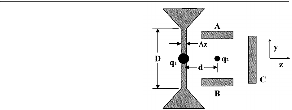
Volume 103, Number 3, May–June 1998

Journal of Research of the National Institute of Standards and Technology

would work. A potential advantage of

ions is that

the axial potential wells required to make

are

not as different as for other choices of ion 2. In a similar

spirit, we could measure the proton (or antiproton)

magnetic moment in terms of other atomic parameters.

For example, the proton spin flip frequency vs

spin

flip frequency could be combined with a separate

measurement of the

spin flip frequency compared

to its cyclotron frequency to yield a measurement of the

proton spin flip frequency to

cyclotron frequency

in the same magnetic field. Coupled with an accurate

value of the electron to

mass ratio, these measure-

ments yield an accurate value of g

. An important

systematic effect to consider in these measurements is

magnetic field inhomogeneity. Field homogeneity could

be checked to high accuracy by moving the

ion to

various locations in the trap, thereby mapping the

magnetic field. Equally important in the proton/antipro-

ton comparison is to insure that the proton and anti-

proton are in the same location. It appears this could be

accomplished by insuring the

is always at the same

location (using optical means) and adjusting the trap

potentials to always yield the same values of

and

1,2

. By this method, it appears that accuracy signifi-

cantly better that 1 part in 10

could be achieved.

6.4 Quantum State Manipulation of Mesoscopic

Mechanical Resonators

Much of what we have discussed concerns manipula-

tion of the mechanical oscillation of atoms or atomic

ions. It is perhaps interesting to speculate on the possi-

bility of applying similar techniques to the manipulation

of macroscopic or mesoscopic mechanical resonators in

the quantum regime [119,120]. If studies can be per-

formed at the quantum level, new sensors at the single

phonon level could be built [324]. One approach is to

make the mechanical resonators small enough and

the temperature low enough that

> k

T [325]; this

approach may obviate the idea discussed here. The idea

we examine here is an extension of the idea of coupling

the oscillatory motion of two ions together; here we

consider coupling the motion of an ion (or the COM

mode of a collection of ions) to a single mode of

mesoscopic mechanical resonator. Although current

technology appears to prohibit performing such experi-

ments at the quantum level, the development of

mesoscopic resonators is rapid and such experiments

may be possible in the future. Similar considerations

regarding coupling of ions to piezoelectric resonators

were discussed in Ref. [48].

To be specific, we consider the situation sketched in

Fig. 13. The mechanical resonator is assumed to be

a silicon beam resonator, fixed at both ends; we will

assume the conditions realized in the experiments of

Cleland and Roukes [325]. The beam resonator has a

length D, thickness in the z direction equal to Dz and a

thickness in the x direction (out of the plane of Fig. 13)

equal to Dx. If we take the conditions of Fig. 3 of

Cleland and Roukes [325] as a guide, we have

D = 7.7 mm, Dz = 0.8 mm, and Dx = 0.33 mm. We

assume that the beam is metalized near its center and

can support a charge q

. For simplicity, we will assume

the metalization is confined to a spherical shell of radius

, but the exact geometry is not so important. Neglect-

ing the dielectric effects of the Si beam (T = 4 K), the

capacitance of the metallized sphere is approximately

equal to C

=4p

. The sphere can therefore support

a charge q

= C

where V

is the potential on the

sphere. An atomic ion of charge q

and mass m

trapped by a combination of electrodes at a distance d

from the cantilever. One of the electrodes is the

charged, metallized sphere; the other electrodes are

indicated schematically as A, B, and C. To estimate the

mass m

of the mechanical resonator we assume it has

a mass equal to half of the beam’s mass and that this

mass is concentrated in the metallized sphere. For the

conditions assumed here, and

(Si) = 2.33 g? cm

–3

,we

find m

≈ 2.4310

–12

g. We arrange the trapping poten-

tials so that the z-oscillation frequency of the ion is

equal to the beam oscillation frequency; in this case, we

realize two coupled oscillators as described in the

previous section. If we take d =5mm, V

= 1000 V,

v¯

/2p = 70 MHz, q

= q(proton), m

=9u (

), we

find from Eq. (155) that t

exch

≈ 6.4 ms. To reliably work

in the quantum regime of the mechanical oscillator, t

exch

Fig. 13. Schematic diagram of an ion coupled to mechanical

resonator. The bridge-type cantilever is essentially the same as that

reported by Cleland and Roukes [325], but is assumed to support a

metallized sphere supporting charge q

.Anionq

is confined by the

potentials on the metallized sphere and additional electrodes shown

schematically as A, B, and C. The Coulomb coupling between the

charges provides the coupling between the two harmonic oscillators.

319

Volume 103, Number 3, May–June 1998

Journal of Research of the National Institute of Standards and Technology

must be smaller than t

, the time for the mechanical

oscillator to make a transition from its un =0l ground

state to the un =1l state. If we assume the conditions of

Cleland and Roukes [325] where T =4K, and

Q =2310

, Eq. (64) gives t

≈ 0.0382 ms. This is

clearly too short to sympathetically cool the beam

resonator’s mode to the ground state, although some

cooling could be achieved as outlined by in Ref. [48]. In

the future, it might be possible to make the ratio t

exch

larger than 1, perhaps through higher Q’s and lower

ambient temperatures [or perhaps if more exotic ion

species with Z

>> 1 become available (Sec. 5.2)], it

may be possible to manipulate the quantum motion of

mesoscopic mechanical resonators by these techniques.

7. Summary/Conclusions

We have attempted to identify some of the important

practical effects which must be taken into account in

order to create arbitrary, entangled quantum states of

trapped ions. We have taken a “passive stabilization”

approach in that we try to anticipate and suggest ways to

guard against the physical effects causing decoherence.

Ultimately, complicated manipulations, such as lengthy

quantum computations, are expected to benefit from

and/or require some form of active error correction.

Indeed, some of the near-term future experiments will

probably demonstrate some of these schemes. In

Sec. IV, we have listed some of the potential sources of

decoherence in trapped ion experiments; here we

speculate on what appear to be the most important of

these.

Motional decoherence is discussed in Sec. 4.1.

In the NIST single

ion experiments [17,21,45,47,

131,132,211], heating appears to be the most important

source of decoherence, primarily because, at the present

time, its source is still unidentified. Various possibilities

were discussed and, although the heating may be caused

by some fundamental effect, we speculate that it is

probably caused by some, as yet undetected, source of

added electric field noise. (Because the current experi-

ments employ electronic filtering at the motional

frequencies, direct observation of fluctuating potentials

on the electrodes has been precluded.) Future experi-

ments will be able to resolve this. Moreover, once this

source of noise is understood, the ion becomes an

extremely sensitive detector of fluctuating potentials

appearing on the electrode surfaces. In any case, it will

probably be desirable to eventually operate the ion

trap at cryogenic temperatures in order to, for example,

reduce the effects of ion loss due to background

gas collisions. A cryogenic environment will have the

added benefit of reducing sources of electronic noise

and associated heating.

Various sources of internal-state decoherence are

discussed in Sec. 4.2. In the current experiments,

decoherence is dominated by fluctuations in magnetic

fields acting on qubit transitions which are strongly field

dependent. It appears that this problem can be highly

suppressed by the use of magnetic shielding and, eventu-

ally, use of qubit transitions which are insensitive

to magnetic field to first order. We expect that internal

state decoherence will be negligible compared to

motional decoherence.

Decoherence induced during application of the logic

pulses (Sec. 4.4) may be the most troublesome. Many of

the sources of this type of decoherence are primarily

technical, for example, caused by intensity fluctuations

in the laser pulses which induce transitions, or

stray light impinging on ions not directly addressed.

The more fundamental causes of decoherence are

(1) coupling to internal or motional states other than the

intended ones (spectator level problem), (2) coupling to

unintended motional modes (cross-mode coupling), and

(3) fluctuations in the Rabi rates due to excitation of the

3L-1 unused motional modes (Debye-Waller factors).

The first two of these effects appear to be a question of

speed. Coupling to unwanted spectator modes and

cross-mode coupling can always be avoided by making

the operations slow enough that the extraneous

couplings are suppressed by spectral selection. This has

the negative effect of allowing more time for decoher-

ence and increasing the required time for a given

computation. Fluctuations caused by fluctuating Debye-

Waller factors are, in principle, reduced as the number

of ions increases because of the averaging effects of

many modes [Eq. (128)]. However, it is also likely that

excitation of these modes is harder to avoid as the

number of ions (and unwanted spectator modes)

increases. It will therefore be desirable to laser-cool all

modes to the zero-point state.

As the number of trapped ions increases, it will be-

come increasingly difficult to avoid these three types of

effects. Therefore, some sort of multiplexing scheme

will be necessary when large numbers of qubits are

involved. In Sec. 5.1, we have presented one possible

solution where the ions are broken up into smaller

numbers of independent groups or registers. The ions

are then connected by moving ions around between

registers. It may also be advantageous to multiplex

quantum information within multiple internal states of

ions; this is briefly described in Sec. 5.2.

Stimulated-Raman transitions between long-lived

qubit states (such as ground-state hyperfine levels) ap-

pear to offer significant advantages over single-photon

optical transitions. Single-photon transitions require

high laser frequency stability, whereas stimulated-

Raman transitions require only high relative frequency

320

Volume 103, Number 3, May–June 1998

Journal of Research of the National Institute of Standards and Technology

stability between the Raman beams, which is techni-

cally easier to accomplish. Stimulated-Raman transi-

tions also provide the ability to select the magnitude and

direction of the effective k vector (k

eff

) by choosing

different directions for the beams. This has the advan-

tage of, for example, allowing k

eff

to be parallel to the

axis of ions in a linear trap, thereby suppressing

coupling to radial modes, while still allowing the Lamb-

Dicke parameter to be controlled by adjusting the angle

of the beams. At the same time, spatial selection of ions

along the axis of the trap can be good since each Raman

beam can be at a relatively steep angle relative to the

trap axis. With single photon transitions, selection of

ions and modes by appropriately choosing the direction

of k can only be obtained for the radial modes in a linear

trap. Stimulated-Raman transitions have the potential

disadvantage of inducing significant ac-Stark shifts

(Sec. 4.4.3). However, for anticipated operating condi-

tions, the effects of Stark shifts can be suppressed

relative to the effects of laser amplitude fluctuations,

which affect both single-photon and stimulated-Raman

transitions.

Decoherence in the ion trap system can probably be

substantially reduced over what has been obtained in

experiments so far. How far this reduction can be carried

is an issue which must be resolved experimentally.

Decohering effects may eventually be controlled to such

a level that fault-tolerant error correction schemes might

be employed to achieve computations of arbitrary

length. This may only require a single operation fidelity

of 10

–5

to 10

–6

[185,326]. If this condition is met, speed

will become an important issue because of the poten-

tially large amount of overhead (increase in number of

required qubits and operations in fault tolerant

schemes). As discussed in Sec. 4.4.6, the Rabi rate for

any operation is limited to approximately the motional

mode frequency. In principle, mode frequencies can be

substantially increased beyond what is currently

achieved (≈ 10 MHz). An obvious direction to pursue is

to make smaller traps with higher trapping potentials;

however, this aggravates the problem of addressability,

and will increase the coupling of the ions to the elec-

trodes thereby increasing decoherence. The optimum

conditions must, again, be resolved experimentally.

8. Appendix A. Entangled States and

Atomic Clocks

We compare the use of entangled vs nonentangled

states in an atomic clock under conditions and con-

straints different than those considered in Sec. 3.4. We

assume that the resources available are a given number

of atoms L and a total observation time which is longer

than any other time scale in the problem. We assume

that decoherence of the internal states is negligible

during the Ramsey free precession time T

.Tomakean

atomic clock, we want to steer, or “lock,” a reference

oscillator ( “local oscillator”) to the atoms’ resonance.

Typically, we can find a local oscillator whose rms

frequency fluctuations D

(

) over short averaging

times

are smaller than the intrinsic fluctuations given

by projection noise. However, for long times, the

frequency fluctuations of the local oscillator are worse

than those given by projection noise. (If this were not the

case, the local oscillator would be a better clock, obviat-

ing the need for the atoms.) By measuring the atomic

populations after each application of the Ramsey radia-

tion [3,9,100], we can generate an error signal which

steers the local oscillator to the center of the atomic

resonance with a servo time constant

. The servo can

make a correction after a few independent measure-

ments on the atoms; for simplicity, we assume

~ T

(Eq. (A4) below). To make the error signal as large as

possible, we want the atomic linewidth D

as small as

possible. The atomic linewidth can be expressed as

= p/(L

–1)

), where

= 1/2 for nonentangled

states and

= 1 for entangled states [3,9,100]. There-

fore, we want T

as large as possible. However, if we

make T

too large, the local oscillator fluctuations

) will be larger than D

, thereby giving no

useful signal. This is the constraint which tells us

whether entangled or nonentangled states are more

useful.

To analyze this problem in detail, we make the follow-

ing assumptions: (1) We assume the (free-running

or unlocked) local oscillator has fluctuations over

averaging time

equal to

(

)=C

. (A1)

This is assumed to hold over the range of values of

which include T

and

. We will consider only values of

n > –1/2, since, for n < –1/2, the local oscillator will

better than the atoms for

sufficiently long. (2) We

assume the intrinsic atomic clock stability, limited by

projection noise, is given by (Sec. 3.4)

meas

(

–

ÏT

, (A2)

(3) For a given servo time constant

, we assume

(

)=K

meas

(

) (A3)

Normally, in the case where D

< D

meas

for short

times

, we would think of adjusting

so that K

< 1;

that is, the local oscillator is locked to the atomic reso-

321

Volume 103, Number 3, May–June 1998

Journal of Research of the National Institute of Standards and Technology

resonance at or before the time

when the local oscil-

lator fluctuations become worse than the projection

noise. However, when K

> 1, the locked local oscillator

stability can eventually reach the stability given by

projection noise (approaching it as 1/

) given adequate

servo gain [327-329]. Therefore we will allow K

to be

larger than 1.

Along with these assumptions, we impose two con-

straints: (1) The servo time constant

must be longer

than the sampling time T

. (We will assume T

is much

larger than the dead time, that is, the time for optical

pumping, detection, etc.) This is expressed by the condi-

tion

= K

, K

> 1. (A4)

For entangled states, each measurement gives one of two

possible values (Sec. 3.4). Therefore, K

must be larger

for entangled states than nonentangled states. (2) For

≈ T

, the atomic linewidth must be greater than the

local oscillator fluctuations or else the error signal used

to correct the local oscillator frequency is ambiguous.

This is expressed by the condition

)=p/(L

–1)

= K

), K

>1.

(A5)

Eq. (A5) gives the sampling time T

as a function of K

–1

n+1

. (A6)

Plugging this into Eq. (A2), we find that the stability of

the locked local oscillator at long times

meas

2(n+1

–

+1/2)

n+1

. (A7)

This is the main result of Appendix A. From this expres-

sion, we see that D

meas

is smaller for entangled states

when n > 0; however, the gain is not as significant as

when we assumed T

to be fixed. We also see that

meas

is smaller for nonentangled states when n <0.

These results are due to the constraint expressed in

Eq. (A5). From the above, we also find

n+1/2

1–

~ K

n+1/2

1–

. (A8)

For nonentangled states on large numbers of atoms, K

and T

are both much larger than for entangled states,

and a very long time may be required to achieve the

intrinsic atomic clock stability given by Eqs. (A2) and

(A7). therefore, as a practical issue, we may wish to

constrain K

to be equal to 1. In that case we find, from

Eqs. (A3) and (A5) two values of R

. We must take the

smaller of these, which results from the value derived

from Eq. (A3) (with K

= 1). Plugging this value of T

into Eq. (A2), we find the stability of the locked oscilla-

tor to be

meas

n+1/2

2(n+1)

–

(2n+1)

2n+2

. (A9)

For large L, entangled states will give a smaller value of

meas

for all values of n > –1/2; however this result is

not fundamental and simply comes from the constraint

that K

is equal to 1.

9. Appendix B. Master Equation for the

Density Matrix of a Radiatively

Damped Harmonic Oscillator

Equation (62) is the master equation for the density

matrix

of a single harmonic oscillator, including

radiative damping terms. This equation is equivalent to

the following system of coupled first-order differential

equations for the diagonal and off-diagonal number-

state matrix elements of

knu

unl ≡

+1)(n+1)

n+1 n+1

–

(2nn

+n+n

)

n–1 n–1

kmu

unl ≡

+1)Ï(m+1)(n+1)

m+1 n+1

Ïmn

m–1 n–1

–

[2n

(m+n+1)+(m+n)]

(B1)

Some special cases of these equations were given in Eq.

(63), where they were used to estimate the time for an

ion to make a transition from the state |0l. Cohen-

Tannoudji [330] treated a similar system, in which the

incoherent excitation was absent (n

= 0), but a

monochromatic perturbation was present. The time

derivative of the thermal average of the number of

vibrational quanta is

322

Volume 103, Number 3, May–June 1998

Journal of Research of the National Institute of Standards and Technology

dkn

≡

n=0

+1)

n=0

n(n+1)

n+1 n+1

–

n=0

–

(2n

+1)

n=0

n=1

n–1 n–1

(B2)

The sums can be simplified to

n=0

n(n+1)

n+1 n+1

n=0

(n+1–1)(n+1)

n+1 n+1

n=0

(n+1)

n+1 n+1

–

n=0

(n+1)

n+1 n+1

n=0

–

n=0

(B3)

and

n=1

n–1 n–1

n=1

[(n –1)

+2n–1]

n–1 n–1

n=1

[(n –1)

+2(n–1)+1]

n–1 n–1

n=0

+1.

(B4)

Collecting terms, we have

n=0

= [

+1) –

(2n

+1)+

]

n=0

–g

+1) –

]

n=0

=–

n=0

(B5)

dkn

=–

. (B6)

In the steady state, kn

l = n

, independent of

(see also,

Ref. [121], p. 97).

Acknowledgments

We gratefully acknowledge the support of the

National Security Agency, the Army Research Office,

and the Office of Naval Research. We thank C. Myatt

and C. Wood for comments and suggestions on the

manuscript. We acknowledge useful discussions with

P. Bardroff, R. Blatt, I. Cirac, T. Darling, L.

Davidovich, A. Despain, D. DiVincenzo, A. Ekert,

B. Esry, N. Gisin, S. Haroche, M. Holland,

M. Holzscheiter, R. Hughes, D. James, J. Kimble,

P. Knight, S. Lloyd, G. Milburn, J. Preskill, W.

Schleich, A. Steane, W. Vogel, P. Zoller, and W. Zurek.

10. References

[1] J. I. Cirac and P. Zoller, Phys. Rev. Lett. 74, 4091 (1995).

[2] C. A. Blockley, D. F. Walls, and H. Risken, Europhys. Lett. 17,

509 (1992).

[3] D. J. Wineland, J. J. Bollinger, W. M. Itano, F. L. Moore, and

D. J. Heinzen, Phys. Rev. A46, R6797 (1992).

[4] J. I. Cirac, A. S. Parkins, R. Blatt, and P. Zoller, Phys. Rev.

Lett. 70, 556 (1993).

[5] J. I. Cirac, R. Blatt, A. S. Parkins, and P. Zoller, Phys. Rev.

Lett. 70, 762 (1993).

[6] H. Zeng, and F. Lin, Phys. Rev. A48, 2393 (1993).

[7] J. I. Cirac, R. Blatt, A. S. Parkins, and P. Zoller, Phys. Rev.

A49, 1202 (1994).

[8] J. I. Cirac, R. Blatt, and P. Zoller, Phys. Rev. A49, R3174

(1994).

[9] D. J. Wineland, J. J. Bollinger, W. M. Itano, and D. J. Heinzen,

Phys. Rev. A50, 67 (1994).

[10] R. Dum, P. Marte, T. Pellizzari, and P. Zoller, Phys. Rev. Lett.

73, 2829 (1994).

[11] H. Zeng, and F. Lin, Phys. Rev. A50, R3589 (1994).

[12] J. Eschner, B. Appasamy, and P. E. Toschek, Phys. Rev. Lett.

74, 2435 (1995).

[13] R. Blatt, J. I. Cirac, and P. Zoller, Phys. Rev. A52, 518 (1995).

[14] H. Zeng and F. Lin, Phys. Rev. A52, 809 (1995).

[15] S. Wallentowitz and W. Vogel, Phys. Rev. Lett. 75, 2932

(1995).

[16] W. Vogel and R. L. de Matos Filho, Phys. Rev. A52, 4214

(1995).

[17] C. Monroe, D. M. Meekhof, B. E. King, W. M. Itano, and

D. J. Wineland, Phys. Rev. Lett. 75, 4714 (1995).

[18] G. Schrade, V. I. Man’ko, W. P. Schleich, and R. J. Glauber,

Quantum Semiclassical Opt. 7, 307 (1995).

[19] R. L. de Matos Filho and W. Vogel, Phys. Rev. Lett. 76, 608

(1996).

[20] R. L. de Matos Filho and W. Vogel, Phys. Rev. Lett. 76, 4520

(1996).

323

Volume 103, Number 3, May–June 1998

Journal of Research of the National Institute of Standards and Technology

[21] D. M. Meekhof, C. Monroe, B. E. King, W. M. Itano, and D.

J. Wineland, Phys. Rev. Lett. 76, 1796 (1996); erratum, Phys.

Rev. Lett. 77, 2346 (1996).

[22] J. F. Poyatos, R. Walser, J. I. Cirac, P. Zoller, Phys. Rev. A 53,

R1966 (1996).

[23] S.-C. Gou and P. L. Knight, Phys. Rev. A54, 1682 (1996).

[24] C. D’Helon and G. J. Milburn, Phys. Rev. A54, R25 (1996).

[25] C. D’Helon and G. J Milburn, Phys. Rev. A54, 5141 (1996).

[26] J. F. Poyatos, J. I. Cirac, R. Blatt, and P. Zoller, Phys. Rev. A54,

1532 (1996).

[27] S. Wallentowitz and W. Vogel, Phys. Rev. A 54, 3322 (1996).

[28] S. Wallentowitz and W. Vogel, Phys. Rev. A55, 4438 (1997).

[29] S.-C. Gou, J. Steinbach, and P. L. Knight, Phys. Rev. A 54,

R1014 (1996).

[30] S.-C. Gou, J. Steinbach, and P. L. Knight, Phys. Rev. A 54, 4315

(1996).

[31] S.-C. Gou, J. Steinbach, and P. L. Knight, Phys. Rev. A55, 3719

(1997).

[32] L. Davidovich, M. Orszag, and N. Zagury, Phys. Rev. A54,

5118 (1996).

[33] M. M. Nieto, Phys. Lett. A 219, 180 (1996).

[34] P. J. Bardroff, C. Leichtle, G. Schrade, and W. P. Schleich, Phys.

Rev. Lett. 77, 2198 (1996).

[35] P. J. Bardroff, C. Leichtle, G. Schrade, and W. P. Schleich, Act.

Phys. Slov. 46, 1 (1996).

[36] J. C. Retamal, and N. Zagury, Phys. Rev. A55, 2387 (1997).

[37] C. C. Gerry, S.-C. Gou, and J. Steinbach, Phys. Rev. A55, 630

(1997).

[38] C. C. Gerry, Phys. Rev. A55, 2478 (1997).

[39] S. Wallentowitz, R. L. de Matos Filho, and W. Vogel, Phys. Rev.

A56, 1205 (1997).

[40] J. I. Cirac, A. S. Parkins, R. Blatt, P. Zoller, Adv. At. Mol. Phys.

37, 237 (1996).

[41] C. S. Adams, M. Sigel, and J. Mlynek, Physics Reports 240,

140 (1994).

[42] P. Berman, ed. , Atom Interferometry, Suppl. 3, Adv. At. Mol.

Phys. (Academic, San Diego, CA, 1997).

[43] P. R. Berman, ed. , Cavity Quantum Electrodynamics, (Aca-

demic, Boston, MA, 1994).

[44] F. Diedrich, J. C. Bergquist, W. M. Itano, and D. J. Wineland,

Phys. Rev. Lett. 62, 403 (1989).

[45] C. Monroe, D. M. Meekhof, B. E. King, S. R. Jefferts, W. M.

Itano, D. J. Wineland, and P. Gould, Phys. Rev. Lett. 75, 4011

(1995).

[46] D. J. Wineland, J. C. Bergquist, J. J. Bollinger, and W. M. Itano,

Physica Scripta, T59, 286. (1995).

[47] C. Monroe, D. M. Meekhof, B. E. King, and D. J. Wineland,

Science 272, 1131 (1996).

[48] D. J. Heinzen, and D. J. Wineland, Phys. Rev. A42, 2977

(1990).

[49] P. S. Jessen and I. H. Deutsch, in Adv. At. Mol. Opt. Phys. 37,

B. Bederson and H. Walther, eds., Academic Press, (1996) p.

95.

[50] M. H. Anderson, J. R. Ensher, M. R. Matthews, C. E. Wieman,

and E. A. Cornell, Science 269, 198 (1995).

[51] C. C. Bradley, C. A. Sackett, J. J. Tollett, and R. G. Hulet, Phys.

Rev. Lett. 75, 1687 (1995).

[52] C. C. Bradley, C. C. , C. A. Sackett, and R. G. Hulet, Phys. Rev.

Lett. 78, 985 (1997).

[53] K. B. Davis, M.-O. Mewes, M. R. Andrews, N. J. van Druten,

D. S. Durfee, D. M. Kurn, W. Ketterle, Phys. Rev. Lett. 75,

3969 (1995).

[54] D. M. Greenberger, M. A. Horne, and A. Zeilinger, Phys. Today

46 (8), 22 (1993).

[55] W. H. Zurek, Progress of Theoretical Physics 89, 281 (1993).

[56] W. H. Zurek, Vistas in Astronomy, 37, 185 (1993).

[57] W. H. Zurek, Physics Today 44, 36 (1991).

[58] A. Garg, Phys. Rev. Lett. 77, 964 (1996).

[59] A. Garg, preprint quant-ph/9710053.

[60] A. Steane, Appl. Phys. B 64, 623 (1997).

[61] D. F. James, Appl. Phys. B 66, 181 (1998).

[62] D. F. James, R. J. Hughes, E. H. Knill, R. Laflamme, and A. G.

Petschek, in Photonic Quantum Computing, S. P. Hotaling and

A. R. Pirich, eds., Proc. SPIE, 3076, (1997) p. 42.

[63] R. J. Hughes, D. F. V. James, E. H. Knill, R. Laflamme, and A.

G. Petschek, Phys. Rev. Lett. 77, 3240 (1996).

[64] R. J. Hughes, D. F. V. James, J. J. Gomez, M. S. Gulley, M. H.

Holzscheiter, P. G. Kwiat, S. K. Lamoreaux, C. G. Peterson,

V. D. Sandberg, M. M. Schauer, C. M. Simmons, C. E.

Thorburn, D. Tupa, P. Z. Wang, and A. G. White, Fortsch.

Phys. 46 (4-6), 329 (1998).

[65] D. J. Wineland, C. Monroe, D. M. Meekhof, B. E. King, and D.

Leibfried, W. M. Itano, J. C. Bergquist, D. Berkeland, J. J.

Bollinger, and J. Miller, in Proc. 15th Int. Conf. on Atomic

Physics, Amsterdam, H. B. van Linden van den Heuvell, J. T.

M. Walraven, and M. W. Reynolds, eds., in World Scientific,

Singapore (1997) p. 31.

[66] D. J. Wineland, C. Monroe, W. M. Itano, B. E. King, D.

Leibfried, D. M. Meekhof, C. Myatt, and C. Wood, Forsch.

Phys. 46 (4-6), 363 (1998).

[67] H. G. Dehmelt, Adv. At. Mol. Phys. 3, 53 (1967).

[68] H. G. Dehmelt, Adv. At. Mol. Phys. 5, 109 (1969).

[69] D. J. Wineland, W. M. Itano, and R. S. VanDyck, Jr. , Adv. At.

Mol. Phys. 19, 135 (1983).

[70] R. C. Thompson, Adv. At. Mol. Phys. 31, 253 (1993).

[71] P. K. Ghosh, Ion Traps (Clarendon, Oxford, 1995).

[72] M. G. Raizen, J. M. Gilligan, J. C. Bergquist, W. M. Itano, and

D. J. Wineland, Phys. Rev. A45, 6493(1992).

[73] J. Drees and W. Paul, Z. Phys. 180, 340 (1964).

[74] M. E. Poitzsch, J. C. Bergquist, W. M. Itano, and D. J.

Wineland, Rev. Sci. Instrum. 67, 129 (1996).

[75] J. J. Bollinger, J. D. Prestage, W. M. Itano, and D. J. Wineland,

Phys. Rev. Lett. 54, 1000 (1985).

[76] J. J. Bollinger, D. J. Heinzen, W. M. Itano, S. L. Gilbert, and

D. J. Wineland, IEEE Trans. Instrum. Measurement 40, 126

(1991).

[77] R. S. Van Dyck Jr. , D. L. Farnham, and P. B. Schwinberg,

Phys. Scrip. T59, 134 (1995).

[78] F. DiFilippo, V. Natarajan, M. Bradley, F. Palmer, and D. E.

Pritchard, Physica Scripta T59, 144 (1995).

[79] G. Gabrielse, D. Phillips, W. Quint, H. Kalinowsky, G.

Rouleau, and W. Jhe, Phys. Rev. Lett. 74, 3544 (1995).

[80] H. Totsuji and J.-L. Barrat, Phys. Rev. Lett. 60, 2484 (1988).

[81] D. H. E. Dubin, Phys. Rev. Lett. 71, 2753 (1993).

[82] J. P. Schiffer, Phys. Rev. Lett. 70, 818 (1993).

[83] T. P. Meyrath and D. F. V. James, Phys. Lett. A 240, 37 (1998).

[84] B. Esry and B. Paul, 1997, unpublished.

[85] R. J. Cook, D. G. Shankland, and A. L. Wells, Phys. Rev. A31,

564 (1985).

[86] M. Combescure, Ann. Inst. Henri Poincare´ 44, 293 (1986).

[87] L. S. Brown, Phys. Rev. Lett. 66, 527 (1991).

[88] R. J. Glauber, in Foundations of Quantum Mechanics, T. D.

Black, M. M. Nieto, H. S. Pillof, M. O. Scully, R. M. Sinclair,

eds., World Scientific, Singapore (1992), p. 23.

[89] R. J. Glauber, in Laser Manipulation of Atoms and Ions,

E. Arimondo, W. D. Phillips, and F. Strumia, eds., North

Holland, Amsterdam (1992), p. 643.

[90] V. N. Gheorghe and F. Vedel, Phys. Rev. A45, 4828 (1992).

324

Volume 103, Number 3, May–June 1998

Journal of Research of the National Institute of Standards and Technology

[91] B. Baseia, R. Vyas, and V. S. Bagnato, Quant. Opt. 5, 155

(1993).

[92] J. I. Cirac, L. J. Garay, R. Blatt, A. S. Parkins, and P. Zoller,

Phys. Rev. A49, 421 (1994).

[93] R. P. Feynman, F. L. Vernon, Jr. , and R. W. Hellwarth, J. Appl.

Phys. 28, 49 (1957).

[94] C. Cohen-Tannoudji, B. Diu, F. Laloe, Quantum Mechanics,

John Wiley and Sons, New York (1977) p. 405.

[95] W. Nagourney, J. Sandberg, and H. G. Dehmelt, Phys. Rev.

Lett. 56, 2797 (1986).

[96] Th. Sauter, R. Blatt, W. Neuhauser, and P. E. Toschek, Phys.

Rev. Lett. 57, 1696 (1986).

[97] J. C. Bergquist, R. G. Hulet, W. M. Itano, and D. J. Wineland,

Phys. Rev. Lett. 57, 1699 (1986).

[98] R. Blatt and P. Zoller, Eur. J. Phys. 9, 250 (1988).

[99] R. J. Cook, in Progress in Optics, XXVIII, E. Wolf, eds., North

Holland, Amsterdam (1990) p. 361.

[100] W. M. Itano, J. C. Bergquist, J. J. Bollinger, J. M. Gilligan,

D. J. Heinzen, F. L. Moore, M. G. Raizen, and D. J. Wineland,

Phys. Rev. A47, 3554 (1993).

[101] D. J. Wineland, J. C. Bergquist, Wayne M. Itano, and R. E.

Drullinger, Opt. Lett. 5, 245 (1980).

[102] H. G. Dehmelt and F. L. Walls, Phys. Rev. Lett. 21, 127 (1968).

[103] D. J. Wineland and H. G. Dehmelt, J. Appl. Phys. 46, 919

(1975).

[104] M. N. Gaboriaud, M. Desaintfuscien, and F. G. Major, Int. J.

Mass Spectrom. Ion Phys. 41, 109 (1981).

[105] K. E. Kahill and R. J. Glauber, Phys. Rev. 177, 1857 (1969).

[106] D. J. Wineland and W. M. Itano, Phys. Rev. A20, 1521 (1979).

[107] E. T. Jaynes and F. W. Cummings, Proc. IEEE 51, 89 (1963).

[108] H. G. Dehmelt, Science 247, 539 (1990).

[109] H. Goldstein, Classical Mechanics, Addison-Wesley, Reading,

MA (1950).

[110] J. Steinbach, J. Twamley, and P. L. Knight, Phys. Rev. A56,

4815 (1997).

[111] J. E. Thomas, P. R. Hemmer, S. Ezekiel, C. C. Leiby, R. H.

Picard, and C. R. Willis, Phys. Rev. Lett. 48, 867 (1982).

[112] W. Happer, Rev. Mod. Phys. 44, 169 (1970).

[113] D. J. Wineland and H. G. Dehmelt, Bull. Am. Phys. Soc. 20,

637 (1975).

[114] D. J. Wineland, R. E. Drullinger, and F. L. Walls, Phys. Rev.

Lett. 40, 1639 (1978).

[115] W. Neuhauser, M. Hohenstatt, P. Toschek, and H. Dehmelt,

Phys. Rev. Lett 41, 233 (1978).

[116] D. J. Wineland, and W. M. Itano, Physics Today 40, (6), p. 34

(1987).

[117] B. Appasamy, I. Siemers, Y. Stalgies, J. Eschner, R. Blatt, W.

Neuhauser, and P. E. Toschek, Appl. Phys. B60, 473 (1995).

[118] G. Morigi, J. I. Cirac, M. Lewenstein, and P. Zoller, Europhys.

Lett. 39, 13 (1997).

[119] V. B. Braginsky and F. Ya. Khalili, Quantum Measurements,

Cambridge University Press, Cambridge (1991).

[120] M. F. Bocko and R. Onofrio, Rev. Mod. Phys. 68, 755 (1996).

[121] D. F. Walls and G. J. Milburn, Quantum Optics, (Springer-

Verlag, Berlin/Heidelberg, 1994).

[122] J. P. Gordon and A. Ashkin, Phys. Rev. Lett. 21, 1606 (1980).

[123] J. Dalibard and C. Cohen-Tannoudji, J. Opt. Soc. Am. B2, 1707

(1985).

[124] H. J. Hope and C. M. Savage, Phys. Rev. A53, 1697 (1996).

[125] D. J. Wineland, J. C. Bergquist, J. J. Bollinger, W. M. Itano, F.

L. Moore, J. M. Gilligan, M. G. Raizen, D. J. Heinzen, C. S.

Weimer, and C. H. Manney, in Laser Manipulation of Atoms

and Ions, E. Arimondo, W. D. Phillips, and F. Strumia, eds.,

North-Holland, Amsterdam (1992), p. 553.

[126] R. L. de Matos Filho and W. Vogel, Phys. Rev. A54, 4560

(1996).

[127] C. K. Law and J. H. Eberly, Phys. Rev. Lett. 76, 1055 (1996).

[128] C. K. Law, J. H. Eberly, and B. Kneer, J. Mod. Opt. 44, 2149

(1997).

[129] S. A. Gardiner, J. I. Cirac, and P. Zoller, Phys. Rev. A55, 1683

(1997).

[130] B. Kneer and C. K. Law, Phys. Rev. A 57, 2096 (1998).

[131] D. Leibfried, D. M. Meekhof, C. Monroe, B. E. King, W. M.

Itano, and D. J. Wineland, Phys. Rev. Lett. 77, 4281 (1996).

[132] D. Leibfried, D. M. Meekhof, C. Monroe, B. E. King, W. M.

Itano, and D. J. Wineland, J. Mod. Opt. 44, 2485 (1997); D.

Leibfried, T. Pfau, and C. Monroe, Phys. Today 51 (4), 22

(1998).

[133] Ch. Kurtsiefer, T. Pfau, and J. Mlynek, Nature 386, 150 (1997).

[134] P. Benioff, J. Stat. Phys. 22, 563 (1980).

[135] P. Benioff, Phys. Rev. Lett. 48, 1581 (1982).

[136] R. Feynman, Int. J. Theor. Phys. 21, 467 (1982).

[137] R. Feynman, Opt. News 11, 11 (1985).

[138] D. Deutsch, Proc. R. Soc. Lond. A400, 97 (1985).

[139] P. Shor, Proc. 35th Ann. Symp. Found. Comp. Sci., IEEE

Computer Society Press, New York (1994) p. 124.

[140] A. Ekert and R. Jozsa, Rev. Mod. Phys. 68, 733 (1996).

[141] A. Barenco, Contemporary Phys. 37, 375 (1996).

[142] A. Steane, Rep. Prog. Phys. 61, 117 (1998).

[143] S. Lloyd, Science 261, 1569 (1993).

[144] S. Lloyd, Science 273, 1073 (1996).

[145] L. K. Grover, Phys. Rev. Lett. 79, 325 (1997).

[146] C. Zalka, Proc. Roy. Soc. Lond., Math. Phys. Sci. (UK) A454,

313 (1998).

[147] S. Wiesner, quant-ph/9603028.

[148] D. S. Abrams and Lloyd, S. , Phys. Rev. Lett. 79, 2586 (1997).

[149] B. M. Boghosian and W. Taylor, Int. J. Mod. Phys. (Singapore)

C8, 705 (1998).

[150] D. A. Lidar and O. Biham, Phys. Rev. E56, 3661 (1997).

[151] S. J. van Enk, J. I. Cirac, and P. Zoller, Phys. Rev. Lett. 78, 429

(1997).

[152] S. J. van Enk, J. I. Cirac, and P. Zoller, Science 279, 205 (1998).

[153] W. G. Teich, K. Obermayer, and G. Mahler, Phys. Rev. B37,

8111 (1988).

[154] G. P. Berman, G. D. Doolen, D. D. Holm, and V. I. Tsifrinovich,

Phys. Lett. 193, 444 (1994).

[155] D. P. DiVincenzo, Phys. Rev. A51, 1015 (1995) and references

therein.

[156] D. P. DiVincenzo, Science 270, 255 (1995).

[157] A. Barenco, D. Deutsch, A. Ekert, and R. Jozsa, Phys. Rev.

Lett. 74, 4083 (1995).

[158] T. Sleator and H. Weinfurter, Phys. Rev. Lett. 74, 4087 (1995).

[159] T. Pellizzari, S. A. Gardiner, J. I. Cirac, and P. Zoller, Phys.

Rev. Lett. 75, 3788 (1995).

[160] P. Domokos, J. M. Raimond, M. Brune, and S. Haroche, Phys.

Rev. A52, 3554 (1995).

[161] P. Domokos, J. M. Raimond, M. Brune, and S. Haroche, in

Laser Spectroscopy, XII International Conf. , Capri, Italy, June

1995, M. Inguscio, M. Allegrini, and A. Sasso, eds., World

Scientific, Singapore (1996) p. 69.

[162] Q. A. Turchette, C. J. Hood, W. Lange, H. Mabuchi, and H. J.

Kimble, Phys. Rev. Lett. 75, 4710 (1995).

[163] W. Lange, Q. A. Turchette, C. J. Hood, H. Mabuchi, and H. J.

Kimble, in Microcavities and Photonic Bandgaps, J. Rarity and

C. Weisbuch, eds., Kluwer (1996) p. 443.

[164] R. To¨rma¨ and S. Stenholm, Phys. Rev. A54, 4701 (1996).

[165] N. A. Gershenfeld and I. L. Chuang, Science 275, 350 (1997).

[166] D. G. Cory, A. F. Fahmy, and T. F. Havel, Proc. Nat. Acad.

Sci.USA 94, 1634 (1997).

[167] V. Privman, I. D. Vagner, and G. Kventsel, Phys. Lett. A239,

141 (1998).

325

Volume 103, Number 3, May–June 1998

Journal of Research of the National Institute of Standards and Technology

[168] D. Loss and D. P. DiVincenzo, Phys. Rev. A57, 120 (1998).

[169] M. F. Bocko, A. M. Herr, and M. J. Feldman, IEEE Trans.

Appl. Supercond. (USA) 7, 3638 (1997).

[170] A. Barenco, Proc. R. Soc. Lond. A449, 697 (1995).

[171] A. Barenco, C. H. Bennett, R. Cleve, D. P. DiVincenzo, N.

Margolus, P. Shor, T. Sleator, J. Smolin, and H. Weinfurter,

Phys. Rev. A52, 3457 (1995).

[172] M. Brune, P. Nussenzveig, F. Schmidt-Kaler, F. Bernardot, A.

Maali, J. M. Raimond, and S. Haroche, Phys. Rev. Lett. 72,

3339 (1994).

[173] N. F. Ramsey, Molecular Beams, Oxford University, London

(1963).

[174] C. Monroe, D. Leibfried, B. E. King, D. M. Meekhof, W. M.

Itano, and D. J. Wineland, Phys. Rev. A55, R2489 (1997).

[175] P. W. Shor, Phys. Rev. A52, R2493 (1995).

[176] A. Steane, Phys. Rev. Lett. 77, 793 (1996); Phys. Rev. A54,

4741 (1996).

[177] A. Steane, Proc. Roy. Soc. Lond. A452, 2551 (1996).

[178] A. R. Calderbank and P. W. Shor, Phys. Rev. A54, 1098 (1996).

[179] R. LaFlamme, C. Miquel, J. P. Paz, and WH. Zurek, Phys. Rev.

Lett. 77, 198 (1996).

[180] A. Ekert and C. Macchiavello, Phys. Rev. Lett. 77, 2585 (1996).

[181] C. H. Bennett, D. DiVincenzo, J. A. Smolin, and W. K. Woot-

ers, Phys. Rev. A54, 3825 (1996).

[182] J. I. Cirac, T. Pellizzari, and P. Zoller, Science 273, 1207

(1996).

[183] D. P. DiVincenzo and P. W. Shor, Phys. Rev. Lett. 77, 3260

(1996).

[184] E. Knill and R. Laflamme, Phys. Rev. A55, 900 (1997).

[185] E. Knill, R. Laflamme, and W. Zurek, Science 279, 342 (1998).

[186] A. Yu Kitaev, Russian Math. Surveys, 1997, to be published.

[187] C. D’Helon and G. J. Milburn, Phys. Rev. A56, 640 (1997).

[188] M. B. Plenio and P. L. Knight, Proc. R. Soc. Lond. A453, 2017

(1997).

[189] D. J. Wineland, J. C. Bergquist, J. J. Bollinger, W. M. Itano, D.

J. Heinzen, S. L. Gilbert, C. H. Manney, and M. G. Raizen,

IEEE Trans. Ultrasonics Ferroelectrics Frequency Control 37,

515 (1990).

[190] D. J. Wineland, J. C. Bergquist, D. J. Berkeland, J. J. Bollinger,

F. C. Cruz, W. M. Itano, B. M. Jelenkovic´, B. E. King, D. M.

Meekhof, J. D. Miller, C. Monroe, and J. N. Tan, in Proc. Fifth

Symp. Freq. Standards and Metrology, J. C. Bergquist, ed.,

World Scientific, Singapore (1996) p. 11.

[191] D. J. Berkeland, J. D. Miller, J. C. Bergquist, W. M. Itano, and

D. J. Wineland, Phys. Rev. Lett. 80, 2089 (1998).

[192] B. Yurke, Phys. Rev. Lett. 56, 1515 (1986).

[193] B. Yurke, S. L. McCall, and J. R. Klauder, Phys. Rev. A33,

4033 (1986).

[194] J. J. Bollinger, D. J. Wineland, W. M. Itano, and D. J. Heinzen,

Phys. Rev. A54, R4649 (1996).

[195] M. J. Holland and K. Burnett, Phys. Rev. Lett. 71, 1355 (1993).

[196] T. Kim, O. Pfister, M. J. Holland, J. Noh, and J. L. Hall, Phys.

Rev. A57, 4004 (1998).

[197] P. Bouyer and M. Kasevich, Phys. Rev. A56, R1083 (1997).

[198] S. F. Huelga, C. Macchiavello, T. Pellizzari, A. K. Ekert, M. B.

Plenio, and J. I. Cirac, Phys. Rev. Lett. 79, 3865 (1997).

[199] J. R. Anglin, J. P. Paz, and W. H. Zurek, Phys. Rev. A55, 4041

(1997).

[200] J. R. Anglin and W. H. Zurek, in Proceedings of the XVI

Moriond Workshop, R. Ansari, Y. , Giraud-He´raud, and J. Traˆn

Thanh Vaˆn, eds., Editions Frontieres (1996) p. 263.

[201] J. A. Wheeler and W. H. Zurek, eds., Quantum theory and

Measurement, Princeton University, Princeton (1983).

[202] D. F. Walls and G. J. Milburn, Phys. Rev. A31, 2403 (1985).

[203] C. M. Savage and D. F. Walls, Phys. Rev. A32, 2316 (1985).

[204] M. J. Collett, Phys. Rev. A38, 2233 (1988).

[205] M. S. Kim and V. Buzˆek, Phys. Rev. A46, 4239 (1992).

[206] P. Goetsch, R. Graham, and F. Haake, Phys. Rev. A51, 3112

(1995).

[207] M. Brune, E. Hagley, J. Dreyer, X. Maiˆtre, A. Maali, C.

Wunderlich, J. M. Raimond, and S. Haroche, Phys. Rev. Lett.

77, 4887 (1996).

[208] G. S. Agarwal, Phys. Rev. A4, 739 (1971).

[209] C. W. Gardiner, Handbook of Stochastic Methods, Springer-

Verlag, Berlin (1983).

[210] D. J. Daniel and G. J. Milburn, Phys. Rev. A39, 4628 (1989).

[211] S. R. Jefferts, C. Monroe, E. W. Bell, and D. J. Wineland, Phys.

Rev. A51, 3112 (1995).

[212] W. Shockley, J. Appl. Phys. 9, 635 (1938).

[213] M. A. Phillip, F. Gelbard, and S. Arnold, J. Coll. Int. Sci. 91,

507 (1983).

[214] G. Gabrielse, Phys. Rev. A29, 462 (1984).

[215] E. C. Beaty, Phys. Rev A33, 3645 (1986).

[216] T. H. Boyer, Phys. Rev. A9, 68 (1974).

[217] S. K. Lamoreaux, Phys. Rev. A56, 4970 (1997).

[218] T. A. Savard, K. M. O’Hara, and J. E. Thomas, Phys. Rev. A 56,

R1095 (1997).

[219] H. Walther, Adv. At. Mol. Phys. 31, 137 (1993); J. W. Emmert,

M. Moore, and R. Blu¨mel, Phys. Rev. A48, R1757 (1993).

[220] C. S. Weimer, F. L. Moore, and D. J. Wineland, Phys. Rev. Lett.

70, 2553 (1993).

[221] R. Alheit, Th. Gudjons, S. Kleineidam, and G. Werth, Rapid

Commun. Mass Spectrometry 10, 583 (1996).

[222] Y. Wang, J. Franzen, and K. P. Wanczek, Int. J. Mass Spec-

trometry Ion Processes 124, 125 (1993).

[223] J. B. Camp, T. W. Darling, and R. E. Brown, J. Appl. Phys. 69,

7126 (1991).

[224] N. Yu, W. Nagourney, and H. Dehmelt, J. Appl. Phys. 69, 3779

(1991).

[225] R. G. DeVoe and R. G. Brewer, in Laser Spectroscopy, M.

Inguscio, M. Allegrini, and A. Sasso, eds., World Scientific,

Sangapore (1996) p. 175.

[226] G. Janik, W. Nagourney, and H. Dehmelt, J. Opt. Soc. Am. B2,

1251 (1985).

[227] J. T. Ho¨ffges, H. W. Baldauf, T. Eichler, S. R. Helmfrid, and H.

Walther, Opt. Commun. 133, 170 (1997).

[228] D. Berkeland, J. D. Miller, J. C. Bergquist, W. M. Itano, and D.

J. Wineland, J. Appl. Phys. 83, 5025 (1998).

[229] Ch. Kleint, Ann. Phys. 10, 309 (1963).

[230] G. W. Timm and A. Van der Ziel, Physica 32, 1333 (1966).

[231] P. A. Redhead, J. P. Hobson, E. V. Kornelsen, The Physical

Basis of Ultrahigh Vacuum, Chapman and Hall, London

(1968).

[232] L. Schmidt and R. Gomer, J. Chem. Phys. 42, 3573 (1965).

[233] F. C. Tompkins, Chemisorption of Gases on Metals, Academic,

London (1978).

[234] L. D. Landau and E. M. Lifshitz, Mechanics, Pergamon, Ox-

ford/New York (1960).

[235] J. C. Bergquist, W. M. Itano, and D. J. Wineland, in Frontiers

in Laser Spectroscopy, T. W. Ha¨nsch and M. Inguscio, eds.,

North Holland, Amsterdam (1994) p. 359.

[236] K. Sugiyama and J. Yoda, Phys. Rev. A55, R10 (1997).

[237] J. B. Hasted, Physics of Atomic Collisions, Butterworth & Co.,

New York (1972).

[238] L. D. Landau and E. M. Lifshitz, Quantum Mechanics—Non-

relativistic Theory, Pergamon, Oxford/NY (1977).

[239] F. G. Major and H. G. Dehmelt, Phys. Rev. 170, 91 (1968).

[240] L. G. Lutterbach and L. Davidovich, Phys. Rev. Lett. 78, 2547

(1997).

326

Volume 103, Number 3, May–June 1998

Journal of Research of the National Institute of Standards and Technology

[241] L. Davidovich, M. Brune, J. M. Raimond, and S. Haroche,

Phys. Rev. A53, 1295 (1996).

[242] J. C. Bergquist, ed., Proc. Fifth Symp. Freq. Standards and

Metrology, World Scientific, Singapore (1995).

[243] P. T. H. Fisk, Rep. Prog. Phys. 60, 1 (1997).

[244] P. T. H. Fisk, M. J. Sellars, M. A. Lawn, C. Coles, A. G. Mann,

and D. G. Blair, IEEE Trans. Instrum. Meas. 44, 113 (1995).

[245] M. Zhu and J. L. Hall, J. Opt. Soc. Am. B10, 802 (1993).

[246] J. Hall, Frequency-Stabilized Lasers and Their Applications,

SPIE Proc. Vol. 1837 (1993) p. 2.

[247] M. Zhu and J. L. Hall, Experimental Methods in the Physical

Sciences, F. B. Dunning and R. Hulet, eds., Academic, San

Diego (1997) p. 103.

[248] F. Plumelle, M. Desaintfuscien, J. L. Duchene and C. Audoin,

Opt. Commun. 34, 71 (1980).

[249] A. A. Madej and J. D. Sankey, Phys. Rev. A41, 2621 (1990).

[250] N. Yu, W. Nagourney, H. Dehmelt, Phys. Rev. Lett. 78, 4898

(1997).

[251] D. A. Church, Phys. Reports 228, 253 (1993).

[252] D. J. Wineland, W. M. Itano, J. C. Bergquist, and F. L. Walls,

in Proc. 35th Ann. Symp. Freq. Control, IEEE, Piscataway, NJ

(1981) p. 602.

[253] W. M. Itano, L. L. Lewis, and D. J. Wineland, Phys. Rev. A25,

1233 (1982).

[254] N. Yu, X. Zhao, H. Dehmelt, and W. Nagourney, Phys. Rev.

A50, 2738 (1994).

[255] W. M. Itano, 1997, unpublished.

[256] H. G. Dehmelt, IEEE Trans. Instrum. Meas. 31, 83 (1982).

[257] D. J. Wineland, W. M. Itano, J. C. Bergquist, J. J. Bollinger, and

J. D. Prestage, Ann. Phys. Fr. 10, 737 (1985).

[258] H. Carmichael, An Open Systems Approach to Quantum Op-

tics, Lecture Notes in Physics m18, Springer, Berlin (1993).

[259] M. B. Plenio and P. L. Knight, Rev. Mod. Phys., 70, 101 (1998).

[260] R. Landauer, in Proceedings of the Drexel-4 Symposium on

Quantum Nonintegrability, D. H. Feng and B-L. Hu, eds., Inter-

national, Boston (1997).

[261] J. F. Poyatos, J. I. Cirac, and P. Zoller, Phys. Rev. Lett. 78, 390

(1997).

[262] I. L. Chuang and M. A. Nielsen, J. Mod. Optics 44, 2455

(1997).

[263] K. Obenland and A. M. Despain, in Proc. 1

NASA Int. Conf.

of Quantum Computing and Quantum Information, to be pub-

lished (quant-ph/9804038).

[264] D. Beckman, A. N. Chari, S. Devabhaktuni, and J. Preskill,

Phys. Rev. A54, 1034 (1996).

[265] A. Barenco, A. Ekert, K.-A. Suominen, and P. To¨rma¨, Phys.

Rev. A54, 139 (1996).

[266] C. Miquel, J. P. Paz, and W. H. Zurek, Phys. Rev. Lett. 78, 3971

(1997).

[267] A. Messiah, Quantum Mechanics, Vol. II North-Holland, Am-

sterdam (1962) p. 744.

[268] J. Lawall and M. Prentiss, Phys. Rev. Lett. 72, 993 (1994).

[269] L. S. Goldner, C. Gerz, R. J. C. Spreuw, S. L. Rolston, C. I.

Westbrook, W. D. Phillips, P. Marte, and P. Zoller, Phys. Rev.

Lett. 72, 997 (1994).

[270] M. Weitz, B. C. Young, and S. Chu, Phys. Rev. Lett. 73, 2563

(1994).

[271] M. Weitz, B. C. Young, and S. Chu, Phys. Rev. A50, 2438

(1994).

[272] N. C. Wong and J. L. Hall, J. Opt. Soc. Am. B2, 1527 (1985).

[273] C. C. Harb, M. B. Gray, H.-A. Bachor, R. Schilling, P. Rotten-

gatter, I. Freitag, and H. Welling, IEEE J. Quant. Elec. 30, 2907

(1994).

[274] S. Schneider and G. J. Milburn, Phys. Rev. A57, 3748 (1998).

[275] R. F. C. Vessot, M. E. Levine, E. M. Mattison, E. L. Blomberg,

T. E. Hoffman, G. U. Nystrom, B. F. Farrel, R. Decher, P. B.

Eby, C. R. Baugher, J. W. Watts, E. L. Teuber, and F. D. Wills,

Phys. Rev. Lett. 45, 2081 (1980).

[276] A. E. Siegman, Lasers, University Science Books, Mill Valley,

CA (1986).

[277] S. Chu (1997) private communication.

[278] J. I. Cirac, P. Zoller, H. J. Kimble, and H. Mabuchi, Phys. Rev.

Lett. 78, 3221 (1997).

[279] H. Frauenfelder, The Mossbauer Effect, Benjamin, New York

(1963).

[280] H. J. Lipkin, Quantum Mechanics, North Holland, Amsterdam

(1973), Chaps. 2-4.

[281] M. A. Kasevich and S. Chu, Phys. Rev. Lett. 69, 1741 (1992).

[282] D. S. Weiss, B. C. Young, and S. Chu, Appl. Phys. B59, 217

(1994).

[283] R. Kosloff, S. A. Rice, P. Gaspard, D. J. Tannor, Chem. Phys.

139, 20 (1989).

[284] S. Shi and H. Rabitz, J. Chem. Phys. 92, 364 (1990).

[285] S. Rice, Science 258, 412 (1992).

[286] W. S. Warren, H. Rabitz, and M. Dahleh, Science 259, 1581

(1993).

[287] J. I. Cirac, R. Blatt, P. Zoller, and W. D. Phillips, Phys. Rev.

A46, 2668 (1992).

[288] R. L. de Matos Filho and W. Vogel, Phys. Rev. A50, R1988

(1994).

[289] M. B. Plenio and P. L. Knight, Phys. Rev. A53, 2986 (1996).

[290] R. A. Cline, J. D. Miller, M. R. Matthews, and D. J. Heinzen,

Optics Lett., 19, 207 (1994).

[291] J. I. Cirac and P. Zoller (1997) private communication.

[292] M. B. Plenio, V. Vedral, and P. L. Knight, Phys. Rev. A55,67

(1997).

[293] H. Harde, H. Lehmitz, J. Hattendorf-Ledwoch, and R. Blatt,

Appl. Phys. B53, 131 (1991).

[294] J. Preskill, Proc. Roy. Soc. Lond., Math, Phys. Eng. Sci. (UK)

A454, 385 (1998).

[295] R. Brewer, R. G. DeVoe, and R. Kallenbach, Phys. Rev. A46,

R6781 (1992).

[296] I. Klaft et al. , Phys. Rev. Lett. 73, 2425 (1994).

[297] J. R. Crespo Lo´pez-Urrutia, P. Beiersdorfer, D. W. Savin, and

K. Widmann, Phys. Rev. Lett. 77, 826 (1996).

[298] R. J. Gould, Astrophys. J. 423, 522 (1994).

[299] A. Einstein, B. Podolsky, N. Rosen, Phys. Rev. 47, 777 (1935).

[300] J. S. Bell, Physics 1, 195 (1964).

[301] J. F. Clauser and A. Shimony, Rep. Prog. Phys. 41, 1881 (1978).

[302] A. Aspect, J. Dalibard, G. Roger, Phys. Rev. Lett. 49, 1804

(1982).

[303] E. S. Fry, T. Walther, and S. Li, Phys. Rev. A52, 4381 (1995).

[304] E. Hagley, X. Maˆtre, G. Nogues, C. Wunderlich, M. Brune, J.

M. Raimond, and S. Haroche, Phys. Rev. Lett. 79, 1 (1997).

[305] D. Greenberger, M. A. Horne, A. Zeilinger, in Bell’s Theorem,

Quantum Theory, and Conceptions of the Universe,

M. Kafatos, ed., Kluwer Academic, Dordrecht (1989).

[306] N. D. Mermin, Am. J. Phys. 58, 731 (1990).

[307] G. C. Ghirardi, A. Rimini, and T. Weber, Phys. Rev. D34, 470

(1986).

[308] P. Pearle, Phys. Rev. A39, 2277 (1989).

[309] S. Wallentowitz, W. Vogel, I. Siemers, and P. E. Toschek, Phys.

Rev. A54, 943 (1996).

[310] G. Drobny´ and B. Hladky´, Acta Physica Slovaka 47, 277

(1997).

[311] B. Buck and C. V. Sukumar, Phys. Lett. 81A, 132 (1981).

[312] P. L. Knight, Phys. Scripta T12, 51 (1986).

[313] K. Banaszek and P. L. Knight, Phys. Rev. A55, 2368 (1997).

327

Volume 103, Number 3, May–June 1998

Journal of Research of the National Institute of Standards and Technology

[314] G. S. Agarwal and J. Banerji, Phys. Rev. A55, R4007 (1997).

[315] C. D’Helon and G. J. Milburn, Phys. Rev. A52, 4755 (1995).

[316] J. J. Slosser and G. J. Milburn, Phys. Rev. Lett. 75, 418 (1995).

[317] F. E. Harrison, A. S. Parkins, M. J. Collett, D. F. Walls, Phys.

Rev. A55, 4412 (1997).

[318] W. K. Lai, V. Buzˇek, and P. L. Knight, Phys. Rev. A43, 6323

(1991).

[319] B. C. Sanders and G. J. Milburn, Phys. Rev. Lett. 75, 2944

(1995).

[320] K. Abdullah, C. Carlberg, E. D. Commins, H. Gould, and S. B.

Ross, Phys. Rev. Lett. 65, 2347 (1990).

[321] M. Charlton, J. Eades, D. Horva´the, R. J. Hughes, and C.

Zimmerman, Phys. Rep. 241, 65 (1994).

[322] W. Quint and G. Gabrielse, Hyperfine Interactions 76, 379

(1993).

[323] D. J. Bate, K. Dholakia, R. C. Thompson, and D. C. Wilson, J.

Mod. Opt. 39, 305 (1992).

[324] M. Roukes (1997) private communication.

[325] A. N. Cleland and M. L. Roukes, Appl. Phys. Lett. 69, 2653

(1996).

[326] A. Steane, quant-ph/9708021.

[327] J. Vanier, M. Teˆtu, and L.-G. Bernier, IEEE Trans. Instrum.

Meas. IM28, 188 (1979).

[328] F. L. Walls, in Frequency Standards and Metrology, Proc. of

Fourth Symposium on Frequency Standards and Metrology,

Ancona, A. DeMarchi, ed., Springer-Verlag, Berlin (1989) p.

145.

[329] J. Dick, J. D. Prestage, C. A. Greenhall, and L. Maleki, in Proc.

21st Ann. Precise Time and Time Interval (PTTI) Applications

and Planning Meeting (1989) p. 487.

[330] C. Cohen-Tannoudji, in Frontiers in Laser Spectroscopy,

R. Balian, S. Haroche, and S. Liberman, eds., North-Holland

(1977), p. 1.

About the authors: David Wineland, Christopher

Monroe, Wayne Itano, and Dawn Meekhof are staff

physicists in the Time and Frequency Division of the

Physics Laboratory at Boulder. Brian King is a gradu-

ate student in physics at the University of Colorado.

Diedrich Leibfried was a guest researcher during

the preparation of the manuscript; he is currently a

physicist at the Institute for Experimental Physics in

Innsbruck, Austria. The National Institute of Standards

and Technology is an agency of the Technology

Administration, U.S. Department of Commerce.

Note added in proof

Some recent experiments are relevant to the subjects

of this paper. In addition to the work at NIST [72,191]

and Garching [219], other groups have realized

Doppler-cooled “arrays” of ions which might be used as

quantum registers [331-335]. The motional modes of

two trapped ions have recently been laser-cooled to the

ground state [336] and differentially addressed to make

approximate Bell states [337]. Recent experiments on

neutral atoms confined in optical lattices have employed

sideband laser cooling using stimulated-Raman transi-

tions [338,339]; these experiments have achieved cool-

ing to kn

l=0 with high efficiency [338,340]. Quantum

state engineering and manipulation, and schemes for

quantum logic will follow [340-342].

References added in proof

[331] R. G. DeVoe and R. G. Brewer, Phys. Rev. Lett. 76, 2049

(1996); Ch. Kurtsiefer and R. G. DeVoe, Abstract, Int. Quant.

Elect. Conf. (1998).

[332] H. C. Na¨gerl, W. Bechter, J. Eschner, and R. Blatt, Appl. Phys.

B66, 603 (1998); H. C. Na¨gerl, D. Leibfried, F. Schmidt-Kaler,

J. Eschner, and R. Blatt, Optics Express, to be published.

[333] W. Alt, M. Block, P. Seibert, G. Werth, Phys. Rev. A (Rapid

Comm.), to be published.

[334] M. Drewsen, C. Brodersen, L. Hornekaer, J. S. Hangst, and J.

P. Schiffer, Phys. Rev. Lett., to be published.

[335] T. B. Mitchell, J. J. Bollinger, D. H. E. Dubin, X.-P. Huang, W.

M. Itano, and R. H. Baughman, submitted for publication.

[336] B. E. King, C. S. Wood, C. J. Myatt, Q. A. Turchette, D.

Leibfried, W. M. Itano, C. Monroe, and D. J. Wineland, quant-

ph/9803023.

[337] Q. A. Turchette, C. S. Wood, B. E. King, C. J. Myatt, D.

Leibfried, W. M. Itano, C. Monroe, and D. J. Wineland, quant-

ph/9806012.

[338] S. E. Hamann, D. L. Haycock, G. Klose, P. H. Pax, I. H.

Deutsch, and P. S. Jessen, Phys. Rev. Lett. 80, 4149 (1998).

[339] H. Perrin, A. Kuhn, I. Bouchoule, and C. Salomon, Europhys.

Lett. 42, 395 (1998).

]340] C. Salomon, private communication.

[341] I. H. Deutsch and P. S. Jessen, Phys. Rev. A57, 1972 (1998).

[342] P. Zoller, private communication.

328